Virtual math

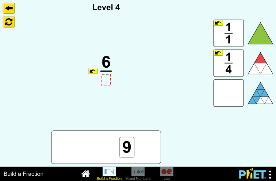
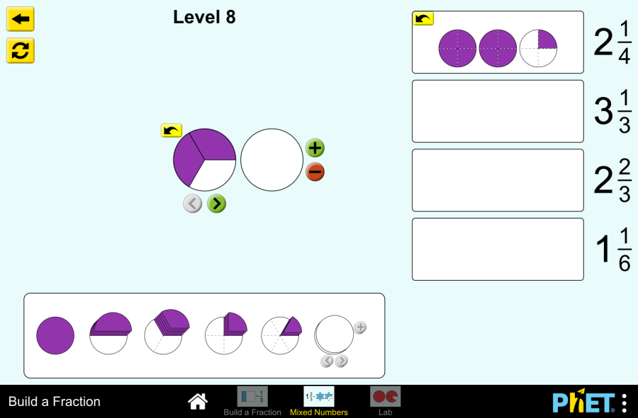
Objective: This virtual work is designed for use in mathematics lessons on the following topics Theoretical part What is a mixed number? Imagine a pizza cut into 8 equal slices. If you eat 3 whole pizzas and 5 more slices from the fourth pizza, how can you keep track of how many pizzas you have eaten? This is where mixed numbers come in. A mixed number has two parts: In our example with the pizza we ate, we’ll write it like this 3 5/8. This reads as “three whole five-eighths”. Example: Why do we use mixed numbers? How do you make an improper fraction into a mixed number? An improper fraction is a fraction where the numerator is greater than the denominator. For example, 11/4. To convert an improper fraction into a mixed number, you must So 11/4 = 2 3/4. Virtual Experiment The Fraction: Mixed Number Simulation allows students to explore and compare different representations of fractions, including mixed numbers. Allows flexibility to explore the correspondence between parts using numbers and representations.  Progression: Part 1. Introduction Step 1. Start the simulation: You will be presented with 3 different modes: “Intro”, “Game” and “Lab”. Open the “Intro” section. Step 2. In the workspace you will be presented with: Step 3. Launch the mixed numbers button. Select the appearance of the fraction according to your needs. Step 4. Click the button that increases the amount of empty skeleton of the fraction model. You will have 2 skeletons.  Step 5. Fill the first skeleton completely and the second skeleton halfway. You will have a mixed number.  Step 6. Increase the size of the fraction. Create different mixed numbers by filling the skeletons. Step 7. Click the button that increases the number of empty skeletons of the fraction model and display some more empty skeletons.  Step 8. Make mixed numbers by collecting and filling the skeletons with different fractions from the shapes. Part 2. Lab Section Step 9. Select the Lab section. You will be given shapes to assemble fractions. You can choose round or rectangular shapes. You are given a blank space to write the fraction and an empty skeleton. Below that are the numbers needed for the numerator and denominator of the fraction.  Step 10. Construct a mixed number from the numbers. Step 11. Arrange the shapes on the empty skeleton according to the given fraction. You can add the necessary number of empty skeletons using the “Add” button. Step 12. You can create a copy in the workspace by dragging the empty space next to the numbers and the empty skeleton next to the shapes. Step 13. Try to collect some mixed fractions. Conclusion Virtual work can be a useful tool for students to become familiar with and understand the concept of mixed numbers. Creating mixed numbers with a visual representation makes it easier to learn the topic.   Glossary of terms

Objective: This virtual activity is designed for use in math lessons on the following topics Theoretical Part What is a part of a whole? Imagine a delicious apple pie. You decide to share it with your friend. What will you do? You cut the pie into two equal pieces. Each of these pieces is a half, or in mathematical terms, 1/2. Fractions and parts Problems to find a part of a whole These are problems where we are given a whole number (for example, the number of apples) and a fraction (for example, 1/4). Our task is to find how many of each number there are (how many apples). For example: There are 12 apples in a vase. Arman ate 1/4 of the apples. How many apples did Arman eat? How do you solve problems like this? Answer: Arman ate 3 apples. Virtual Experiment In this virtual activity, students play games to build fractions from parts of different shapes. Some of the problems are number problems, while others are visual problems. Course of work: Part 1. Learning to build correct fractions Step 1. Start the simulation: You will be given 3 different modes: “Build a Fraction”, “Mixed Numbers”, “Lab”. Choose the “Build a Fraction” section.  Step 2. You will be given different levels. On the levels given by fractions, the figures are represented as numbers, and you will build fractions from the figures. And on the levels given by numbers, the fractions are shown as shapes, which you will use to write fractions with numbers. Choose one of the given levels. Step 3. On the right side of the screen the fractions to be collected are listed. You can collect these fractions in the middle. And the bottom part lists the items to assemble the fractions. On the left side, there are Back and Restart buttons. Step 4. Compose the first type of fractions.  Step 5. To check the correctness, left-click and drag the mouse over the space next to the given fraction. If the fraction is assembled correctly, it will be placed in the space, and if an error occurs, the fraction will be returned to its place of assembly. Step 6. Assemble the other types of fractions as well.  Step 7. If you have done everything correctly, you can go to the next level and perform the other given fractions. Or you can go back to the levels section and choose another level by clicking on the “Back” button in the top left corner. Part 2. Learning to create mixed fractions Step 8. Select the Mixed Numbers section. You will be presented with different levels as in the “Build a Fraction” section. Choose one of them.  Step 9. Build the first type of fraction. Place it by dragging it into the empty space next to the given fraction. If an error occurs, the fraction will be returned to the place where it was built. Step 10.  Build the other types of fractions.  Step 11. Once you have done this correctly, you can perform other given fractions by advancing to the next levels. Conclusion Students will improve their knowledge of simple fractions, mixed numbers, by performing tasks in this simulation. It can be a useful tool in learning to solve problems related to fractions. Glossary of terms

Objective: This virtual work is designed for use in mathematics lessons on the following topics Theoretical part Problems to find the whole from parts In these problems we are given a part of a whole and we know what that part is. Our task is to find this whole. Example: Nazgul has 5 apples. This is 1/3 of all the apples in the basket. How many apples are in the basket? Answer: Comparing and balancing fractions and mixed numbers Compare fractions: Compare mixed numbers: First compare the whole numbers. If they are equal, compare the fractional parts. Criteria for making fractions equal Virtual Experiment In the Aligning Simple Fractions virtual experiment, students learn to find and align fractions using numbers and pictures. Performs fraction calculations in a fun way to easily master the topic of simple fractions. Align the same fractions using different numbers and fraction representations. Progression: Part 1. Play with correct and incorrect simple fractions Step 1. Start the simulation: You will be presented with 2 different modes: “Fraction” and “Mixed Numbers”. Open the “Fraction” section. Step 2. In the workspace you will be presented with 8 different levels of problems. Levels 1-2 use less than 1 fraction. Levels 3-6 use fewer than 2 fractions. Levels 7-8 use only more than 1 and less than 2 fractions.  Step 3. Open the first level. In the work area you are provided with:  Step 4. Bring any fraction to the scales by left-clicking and dragging it.  Step 5. Among the remaining fractions, find a fraction that is equal or proportional to the fraction on the scale. Place it on the second scale.  Step 6. Check for correctness by clicking on the “Check” button. If the fractions are equal, click “OK” and perform the next alignment. If there is an error, click “Try again” and align the fractions from the beginning.  Step 7. Complete the tasks in a level and move on to the next level. Part 2. The Mixed Numbers Game Step 8. Open the “Mixed Numbers” section. In the workspace, you will see 8 different levels of problems. Levels 1-6 use less than 2 mixed number fractions. Levels 7-8 use more than 1 and less than 2 fractions. Step 9. Open the first level. This section also provides a workspace like the first section. This is where you will do mixed number problems. Step 10. Move any fraction to the scales by left-clicking and dragging. From the remaining fractions, find one that is equal to or proportional to the fraction on the scale. Place it on the second scale. Check your work by clicking on the “Check” button.  Step 11. Complete the tasks of one level and move on to the next levels.  Conclusion In this simulation, students used the basic property of fractions to reduce fractions by comparing and making fractions equal to each other. Understanding the equality of fractions can be the basis for further learning about fractions and performing various mathematical operations with them.

Objective: This virtual activity is designed to be used in math lessons in the next chapter: Theoretical Part A quadrilateral is a special case of a polygon with four sides and four vertices. Classification of quadrilaterals Properties of Rectangles Virtual experiment In the “rectangles” simulation, students explore the properties and relationships between named square figures. Workflow: Step 1. In the work area you are provided with: Step 2. Activate the marker, grid, diagonals buttons. Marker, grid buttons help to compose the figure, diagonal button explore the diagonals of the figure. Step 3. Build a rectangle from the given rectangle. To do this, you move the desired quantity by holding each of the points A, B, C, D. Check the correct figure by including a board with the name of the rectangle. The name is rectangle. Examine the diagonals of the figure. Step 4. Construct a square. The name – square appears on the board. Study the diagonals of the shape. Step 5. Press the Restore Initial View button each time to simplify the creation of each shape. Step 6. Build a rhombus. The name on the board is Rhombus. Study the diagonals of the figure. Step 7. Build a trapezoid with one 90-degree angle. The name on the board is trapezoid. Study the diagonals of the figure. Step 8. Construct an isosceles trapezoid. The name isosceles trapezoid appears on the board. Examine the diagonals of the figure. Step 9. Construct a parallelogram. The name on the board is parallelogram. Study the diagonals of the figure. Step 10. Other compound rectangle types refer to convex rectangles. Try to construct convex rectangles of different shapes. The name on the board is convex quadrilateral. Step 11. Construct a kind of rectangle in which at least one of the interior angles is greater than 180 degrees. This is a concave quadrilateral. The name on the board is concave quadrilateral.  Conclusion This virtual activity allows students to explore the types and diagonals of a rectangle. It is used as an aid to explore the similarities and differences of figures in geometry lessons. Glossary of terms

Objective: This virtual activity is designed to be used in math lessons on the following topics: Theoretical part A fraction is a number that shows how many equal parts a whole is divided into and how many such parts are taken. For example: The structure of a fraction A fraction consists of two numbers written on top of each other and separated by a line: For example: In the fraction 3/4, the number 3 is the numerator and the number 4 is the denominator. Proper and improper fractions Fractions are divided into two types: Virtual Experiment Modeling the construction of a fraction allows students to predict and understand how changing the numerator of a fraction affects its value, and how changing the denominator of a fraction affects its value. Allows flexibility to explore the correspondence between parts using numbers and pictures.  Workflow: Step 1. Start the simulation: You will be presented with 3 different modes: “Intro”, “Game” and “Lab”. Open the “Intro” section. Step 2. In the workspace you will be presented with Step 3. On the empty fraction model frame, move your mouse over the shape that makes up the fractions. You will also see that the numerator of the fraction is equal to 1 in the denominator. That is, the fraction 1/1 – forms a complete shape. The type of fraction is an improper fraction. Step 4. Increase the fractional part by 2. You get ½, which is half of the shape. Therefore, it appears that ½ represents half of the shape. The type of fraction is a proper fraction. Step 5. Increase the fractional part by 3. You get a part of ⅓. This type of fraction is a proper fraction. Step 6. Increase the numerator of the fraction by 2. You get a fraction of 2/3. This type of fraction is a proper fraction. Step 7. So, you can find out what a fraction shape looks like by increasing or decreasing the numerator and denominator of the fraction. Try making different types of fractions. Step 9. Build improper fractions by collecting empty skeletons from different fractions.  Step 10. You can repeat the experiments for other types of shapes.  Conclusion This virtual activity reinforces students’ knowledge of fractions. The simulation shows how fractions are shaped and helps students to better understand the concept of fractions. Glossary of terms

Objective: This virtual activity is designed for use in the math lessons in the following chapter:  Theoretical Part What is an equilibrium? Imagine you are standing on one leg. In order not to fall, you have to keep your body straight. That’s what balance is! When all the forces acting on you are balanced, you are standing straight. Properties of balance The lever has the same function as a large scale. When you place objects on it, it can tilt to one side or the other. Why does this happen? It depends on the weight of the objects and how far they are from the center of the board. How can you predict what will happen to the lever? Virtual Experiment In a virtual activity, students play by placing objects on a lever to learn about balance. Explore equating the lever with different substances to determine the mass of mystery objects. Guesses which direction the lever is moving when supports are removed. Solve balance puzzles. As the level increases, the puzzles become more difficult. Progression: Step 1. You are given 3 different modes, “Intro”, “Balance Lab” and “Game”. Open the “Balance Lab” section. Balance Lab Section Step 2. In the work area provided to you: Step 3. Remove the frame. Level, add markers to measure the distance from the pivot point. Step 4. Place objects of the same mass at the same distance on the arm (the object is a brick). Step 5. Place objects of different masses at the same distance on the lever. (Object – People) Step 6. Place people on the lever, the mass of one is twice the mass of the other. Let the person with the greater weight be twice as close to the fulcrum.  Step 7. Use comparisons to level the mystery objects by placing them on the lever. Game Section Step 8. Open the “Game” section. You will be given four levels. Open one level. Step 9. You will be given tasks to align the lever, determine what happens when the support or body weight is removed. Once you have completed the task, you will move on to the next. Step 10. On one level you will be given 6 tasks. Once you complete them, you can move on to the next levels.  Conclusion Students have learned many interesting things about balance. To keep a lever in balance, you have to consider not only the weight of the objects, but also how far they are from the center.

Objective: This virtual work is intended for use in algebra lessons on the following topics Theoretical Part The equation of a line in the form y – y1 = m(x – x1) is called the point angle form. This equation describes a line passing through a given point M1(x1, y1) with a given angular coefficient (slope) m. The geometric significance of the parameters: m (angular coefficient): (x1, y1): The coordinates of the point M1 through which the line passes. This point always belongs to the line. How to use the point angle form? Graph construction: Write the equation: Relation to other forms of the equation of a straight line: Virtual Experiment In this virtual activity, students graph a straight line given an equation such as y – y1 = m(x – x1). Investigates the parameters of a linear equation in the form y – y1 = m(x – x1). Predicts how changing the values in the linear equation will affect the line shown on the graph. Course of Work: Part 1. “Slope Intercept” Step 1. You will be given 4 different modes, “Slope”, “Slope-Intercept”, “Point-Slope”, and “Line game”. You will work in the “Point-Slope” and “Line game” sections. Start the “Point-Slope” mode. Step 2. You are given:  Step 3. Set the points on the graph using the tools that display the values of the points (x, y) in the graph coordinates. Add buttons to display the graphs of y = x and y = – x. Examine the graph. You will see that the equation y-2 = ¾ (x-1) intersects the equation y = x at point (5,5). Step 4. Control the purple and blue dots to change the equation. Drag the purple point to see how the point changes in the equation. Drag the blue point to change the slope. Examine the graph. Step 5. In addition to changing the points, you can control the equation by changing the parameters of the function y – y1 = m(x – x1). Change the settings and examine the graph.  Part 2. “Line game” Step 6. Activate the “Line game” mode. You are given 6 levels. In this activity you will work on levels 1 to 4. Select the first level. Step 7. You are given  Step 8. You have an equation or graph in green. This is the task you must complete:  Complete and review the assigned problem.  Step 9. Complete the assignment and move on to the next level.  Conclusion The virtual lab is a valuable tool for students to learn the graphs of linear functions. The simulator has become interactive and visually useful by providing various tools for learning graphs, such as displaying points, displaying equations, and saving graphs.

Objective: This virtual work is intended for use in algebra lessons on the following topics Theoretical part The slope of a graph, or angle coefficient, shows how steeply the line rises or falls. It is a key parameter for describing linear functions and has many practical applications. Formula for Calculating the Slope The following formula is used to calculate the slope of a line passing through two points (x₁, y₁) and (x₂, y₂): m = (y₂ – y₁) / (x₂ – x₁), where: What the slope means: How to use the formula: Virtual Experiment In the Slope Screen simulation, students explore the parameters of the slope formula and how changing the graph affects the equation or how changing the equation affects the graph. Course of Work: Part 1. “Slope” Step 1. You are given 4 different modes, “Slope”, “Slope-Intercept”, “Point-Slope”, and “Line game”. You will work in the “Slope” and “Line Game” sections. Start the “Slope” mode. Step 2. You are given:  Step 3. Determine the points on the graph using the tools that display the point values (x, y) in graph coordinates. Examine the slope equation. Step 4. Change the values of (x₁, y₁) and (x₂, y₂) from the slope equation. Examine the graph.  Step 5. Save the graph type, make some more graphs, and make comparisons with the slope equations. Part 2. The Game Part Step 6. Activate the “Line Game” mode. You will be given six levels. In this activity, you will work on levels five and six. Select the fifth level. Step 7. You are given  Step 8. You have an equation or graph in green. This is the task you must complete:   Complete and review the assigned problem.  Step 9. Complete the assignment and move on to the next level.  Conclusion This virtual work is a slope formula for linear functions for students and a valuable tool for learning graphs. The simulator has become interactive and visually useful by providing various tools for learning graphs, such as displaying points, displaying equations, and saving graphs.

Objective: This virtual activity is designed to be used in math lessons in the next chapter: Theoretical part When we add numbers, we combine their quantities. Imagine that you have 25 apples and your friend has 32. To find out how many apples you have together, you have to add the two numbers. Digitizing numbers Column Addition Algorithm When numbers become large, it can be difficult to add them mentally. For such cases, we use the column addition method. We write the numbers below each other so that the units are below the ones, the tens below the tens, and the hundreds below the hundreds. Begin addition by adding units. If the sum of the units is less than 10, write the result below the line in the unit place. If the sum of the units is 10 or greater, write only the units of the result and move the tens to the next place (tens). Add the tens, remembering to add the carry (if there was one). Write the result below the line in the tens place. Add the hundreds. Write the result below the row in the hundreds. Virtual Experiment The Explore screen allows students to focus on place value, addition strategies, and even subtraction as they learn to combine and divide numbers. Teachers can use this screen as a tool for explaining numbers. On the Play screen, students complete tasks that develop integration skills. Workflow: Step 1. There are 3 different modes: “Explore”, “Adding” and “Game”. Open the “Explore” section. Explore Section Step 2. In the workspace provided to you: Step 3. Divide tens by units. You can divide by units by clicking and dragging the specified hand.  Step 4. Subtract and add some tens and units on the screen. You subtract by holding the top of the cards with the number written on them and add by holding the bottom. Step 5. Extract and add some hundreds, decimals, and ones to the screen. In order, add the hundreds first, followed by the tens and then the ones. Adding Section Step 6. Open the Adding section.  Step 7. Enter two additions of numbers. If you press the Pencil and Page button, a calculator will appear on the screen. Enter the number and click the “Submit” button. Step 8. Find the value of the sum by holding one connector and dragging it over the other.  Game Section Step 9. Open the “Game” section. You will be given 10 levels of addition problems. Open the first level. Step 10. Write down the number of points given on the screen.  Step 11. Go to the next problem and solve it. There are 10 problems in each level. When you are done with the problems, move on to the problems of the next level. Conclusion Adding two-digit numbers and hundredths is an important skill that will come in handy in later math studies. Constant practice helps students to perform such tasks quickly and confidently. The simulator can be a special visual aid for a better understanding of the subject.

Objective: This virtual activity is designed to be used in the algebra lesson in the next chapter: Theoretical part Plinko is a fascinating combination of chance and mechanics. A ball passing through many nails will eventually fall into one of the lower slots. It seems impossible to predict exactly where the ball will fall. However, the mathematical apparatus allows us to get closer to answering this question.  Average: This is the standard arithmetic mean. It shows what value our data is clustered around. In our game, this would be the average number of cells the ball passes through to the end. Dispersion: This shows how much our data is scattered around the mean. A large variance means that the results are very different from each other. Standard deviation: This is the square root of the variance. It tells us how much our data varies on average from the mean. Binomial Distribution: This is a probability distribution that describes the number of successes in a sequence of independent trials, each with only two possible outcomes (e.g., the ball deflects left or right). In our Plinko game, we can use the binomial distribution to model the process of dropping the ball. Binomial distribution formula: x=(x1+x2+…+xn)/n σ = √[ Σ(xᵢ – x̄)² / (n – 1) ] μ = (Σx) / N smean=s / μ Virtual Experiment The main purpose of our work is to experimentally confirm the theoretical knowledge about mean, variance and standard deviation using the example of the Plinko game in the Phet simulation. In this work, students can predict which basket the ball will fall into and compare several trials. They can further explore binary probability using the parameters on the board. Workflow: Step 1. You will be given 2 different modes, “Intro” and “Lab”. Open the “Lab” section. Step 2. In the workspace you are provided with Step 3. Switch the ball flow to continuous.  Step 4. Start the game. Stop when the balls reach a certain number. Step 5. Examine the data. See the mean, standard deviation values, arithmetic mean. How to be in perfect condition. Try converting the number of balls in the cells to a fractional type. Step 6. Change the number of rows, binary probability. Step 7. Restart the game. Examine the data. Compare the results of the game with the previous probability distributions. Conclusion The use of the simulator allowed us to visualize the relationship between probability theory and concrete experiments. The theoretical ideal calculated the mean and compared the standard deviation that we get from several experiments on the simulator. We verified that the results depend on changing the game settings.