Virtual math

Objective: This virtual activity is designed to be used in math lessons in the next chapter: Theoretical part A ratio is a comparison of two quantities. It shows how many times one quantity is greater or less than the other. A ratio is written as a fraction or with a colon. For example, the ratio of the number of apples to the number of pears is 3:5, which means that there are 1.67 times fewer apples than pears. Proportion is the equality of two ratios. It is written as two fractions separated by an equal sign. For example, 3/5 = 6/10 is a proportion. Proportions are widely used to solve various problems related to the proportional dependence of quantities. Basic properties of proportions: Virtual experiment In this activity, you can play directly with the fluidity values and get immediate feedback as an illustrated relationship.  The second screen has an additional control that allows students to make predictions before seeing their aspect ratios.  Each context provides a unique but rich environment for exploring ratios. Students will naturally want to explore each context and can focus on what they like best until they are asked to focus on something specific. Workflow: Step 1. You are given 2 different modes, “Explore” and “Predict”. Open the “Explore” section. Step 2. In the workspace you are provided with Step 3. Create a bead necklace. Create different proportions with red and blue beads. Step 4. Select a type of bead to create a proportion. Here, blue and yellow, red and yellow, and black and white beads are mixed in different ratios to create proportions. Step 5. Give the number of blue and yellow beads and create a ratio. Continue to make predictions about the relationship by looking at the color scheme.  Step 6. Select the type of pool table. This is where you create relations by giving the board different lengths and widths.   Step 7. Choose the type of apple. This is where you evaluate apples. You will see the relationship. Activate the “Show apple price” button. Step 8. Enter the number of apples and the price. This way you can see their relationship. Step 9. Open the “Predict” section. The workspace looks like the “Explore” section. Here you make an assumption about what the ratio will be by looking at the number of two items the ratio is involved in. Step 10.  Make a prediction about the type of necklace based on the number of beads. Check your guess by clicking the “eye” button.  Step 11. Mentally make different necklaces by transferring the number of beads in different ways. Keep checking to see if your prediction is correct.  Step 12. Try working with types that create proportions. Conclusion By creating this virtual activity, students will be convinced that proportions and ratios are not difficult math problems, but an interesting topic with many real-life examples.

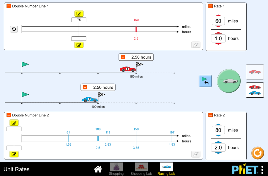
Objective: This virtual activity is designed to be used in the math lessons in the next chapter: Grade 6. “Dependence between quantities”  Theoretical part Direct proportionality is a relationship between two quantities in which an increase in one quantity by a factor of several leads to an increase in the other quantity by the same factor. In other words, the ratio of these quantities always remains constant. Example: Speed and distance traveled: The faster you go, the farther you go in the same amount of time. Direct Proportionality Formula y = kx, where: y and x are two directly proportional quantities, k is the coefficient of proportionality, which indicates how many times y increases when x is increased by 1. Virtual Experiment In this simulation, students create reports about the relationship between quantities. The Racing Lab screen allows students to compare speeds on a racetrack. Students can examine roads of different lengths and cars of different speeds. Identifies the unit rate and how it is calculated. Develop strategies for using unit rate to solve problems.  Workflow: Step 1. You will be given 3 different modes, “Shopping”, “Shopping Lab” and “Racing Lab”. In this activity you will work in the “Racing Lab” section. Open the “Racing Lab” section. Step 2. In the workspace, you will find Step 3. Set the speed of the car. Step 4. Drive the car. Check the data.  Step 5. Press the button to output two roads and cars to the screen. Give the cars different speeds. Make the finish point the same for both cars.  Step 6. Drive the cars. Examine the data.  Step 7. Do some more experiments and run the study. Conclusion  In this activity, students solved problems about the relationship between quantities. They found the relationship between speed, distance, and time. They compared these quantities for two simultaneous cases.

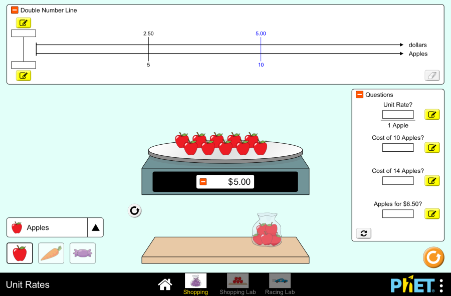
Objective: This virtual activity is designed to be used in math lessons in the next chapter: Theoretical Part Dependence between quantities: In the world around us, many quantities are related to each other. For example: A dependency is a relationship between two or more quantities in which a change in one quantity causes a change in the other. Ways to Convey Dependencies There are several ways to communicate a dependency between quantities: Example: “The price of an apple is 20 tenge per kilogram.” Create a formula based on the description Virtual Experiment In this simulation, students create reports about the relationship between quantities. As they shop for fruits, vegetables, and candy, they learn about the unit price. Identifies the unit rate and how it is calculated. Develop strategies for using the unit rate to solve problems. In the Shopping Lab, students can set prices directly.  Workflow: Step 1. You will be given 3 different modes, “Shopping”, “Shopping Lab”, and “Racing Lab”. In this activity, you will work in the first two sections. Open the “Shopping section”. Shopping Section Step 2. In the workspace, you will be provided with Step 3. Place the orange on the scale.  Step 4. Create reports on the taskbar based on the data. You can leave the desired number of oranges on the scale or add more oranges. Examine the data on a double numeric scale.  Step 5. You can refresh the Tray and create more reports related to orange.  Step 6. Replace the orange with another fruit, vegetable, or candy. Complete the tasks. Shopping Lab Section  Step 7. Open the Shopping Lab section. In the workspace, you will find Step 8. Set the price of an apple. Place the apples on the scale.  Step 9. Enter the number of apples on the two-digit scale. Calculate and record the corresponding price. Step 10. You can do several experiments in the lab by changing the two-digit scale, the price, or the apple.  Conclusion Students have learned about relationships, the dependence between quantities, by working on this simulation. The topic has been illustrated by calculating the price of a good and its quantity.

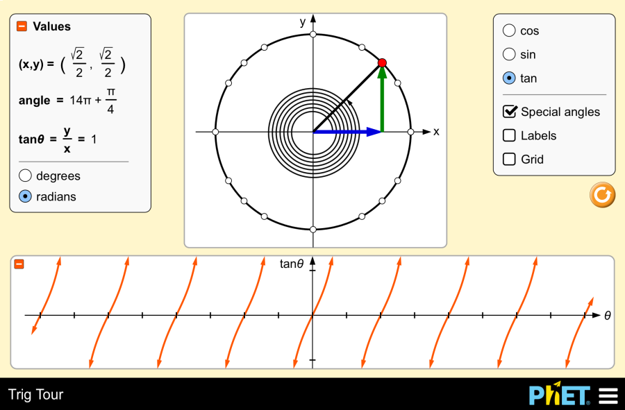
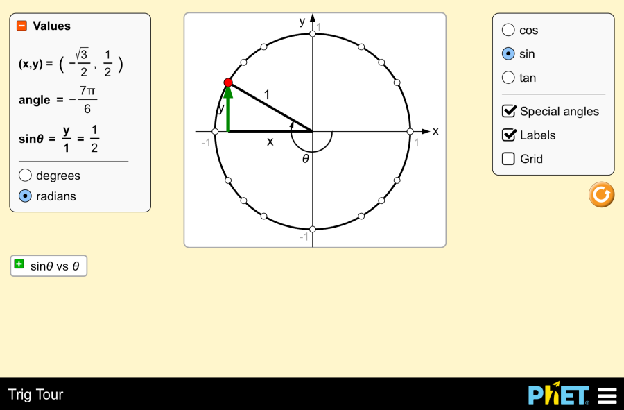
Objective: This virtual activity is designed to be used in the algebra lesson in the next chapter: Theoretical Part Properties of trigonometric functions For sine and cosine, the definition domain is all real numbers and the value domain is the interval [-1, 1]. For tangent and cotangent, the domain is all real numbers except the points where cosine and sine converge to zero, respectively. The range of values is all real numbers. Graphs of Trigonometric Functions Graphs of trigonometric functions allow us to visualize their properties. Virtual Experiment The Trig Tour simulator allows students to find the graphs of trigonometric functions, estimate or find the real values of trigonometric functions, and derive the signs of trigonometric functions ( + , -, 0) for any given angle without a calculator. Workflow: Step 1. Launch the simulator. In the workspace, you will see Step 2. Activate buttons special angles, labels. Step 3. When the angle is 0⁰, examine cos α. Value range [-1, 1]. The range of definition is all real numbers. Period 2π. Step 4. Change the degrees of the angle to special angles and learn cos θ. Try changing the degrees to radians. Step 5. Change the trigonometric function to sine. When the angle is 0⁰, examine sin α. Range of values [-1, 1]. The domain is all real numbers. The period is 2π. Step 6. Switch to special angles and study sin θ. Step 7. Change the trigonometric function to tangent. If the angle is 0⁰, examine tg θ. The range of values is all real numbers. The tangent is defined for all angles except those that are multiples of π/2 (90 degrees) plus or minus any integer π. Period π. Step 8. Switch to special angles and examine the tangent θ. Step 9. Uncheck the special angles and examine the functions. Conclusion The student worked in a simulation and studied the graph of a function as a function of angle and the numerical values of the function as the side of a right triangle inscribed in a unit circle. Using the concept of the unit circle, he determined the sign of the trigonometric function ( + , -, 0) for any given angle without a calculator. Using the concept of the unit circle, he estimated the value of trigonometric functions for any given angle without a calculator.

Objective: This virtual activity is designed to be used in the algebra lesson in the next chapter: Grade 9. “Sine, cosine, tangent, and cotangent of an arbitrary angle. Values of sine, cosine, tangent and cotangent of angles”.  Theoretical Part The basic trigonometric functions are sine, cosine, tangent, and cotangent. These functions establish the relationship between the sides and angles of a right triangle. For a deeper understanding of trigonometric functions, it is convenient to use the unit circle – a circle of radius 1 centered on the origin. Any point on this circle defines an angle with a positive direction from the positive half axis Ox. The coordinates of this point are equal to the cosine or sine of this angle. Definitions of the trigonometric functions: The values of trigonometric functions for some angles (0°, 30°, 45°, 60°, 90°, etc.) are often used in various calculations. These values can be found in special tables or calculated with a pocket calculator. Virtual Experiment In this activity, students estimate the value of trigonometric functions for any given angle without a calculator using the concept of a unit circle. Identifies specific trigonometric functions for given angles, using degrees or radians to measure angles. Workflow: Step 1. Launch the simulator. In the workspace, you will see Step 2. You don’t need the function graph. Assemble it. Activate buttons special angles, labels. Step 3. When the angle is 45⁰, examine cos θ. Cosine (cos θ): the ratio of the length of the adjacent leg to the length of the hypotenuse. Step 4. Change the degrees of the angle to special angles and explore cos θ. Try changing the degrees to radians. Step 5. Change the trigonometric function to sine. Sine (sin θ): the ratio of the length of the opposite leg to the length of the hypotenuse. Step 6. Switch to special angles and examine sin θ. Step 7. Change the trigonometric function to tangent. Tangent (tg θ): the ratio of the length of the opposite leg to the length of the adjacent leg. Step 8. Switch to special angles and study tg θ. Conclusion Students used the simulator to calculate the values of trigonometric functions of angles given in degrees (radians), which are often used in practice. Learning trigonometric functions by sight in a unified structure can be a good aid to understanding the subject.

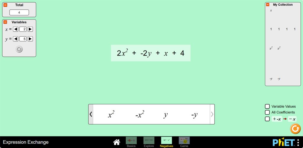
Objective: This virtual activity is designed to be used in math lessons in the next chapter: Theoretical part Definition and representation Examples: Operations on positive and negative numbers Addition: For example, -12+(-3)=-15; -7+9=2. Subtraction: For example, 18-(-23)=41. Virtual Experiment In this virtual experiment, students learn how to reduce an expression. Create complex expressions that may involve subtraction and negative variable values. Creates expressions that match the tasks in the Games section.  Plays with variables in Levels 5-8. Levels 7-8 include division problems. Workflow: Step 1. Launch the simulation. There are 4 different modes. “Basics”, “Explore”, “Negatives” and “Game”. You will work in the “Negatives” and “Game” sections. Open the “Negatives” section. Step 2. In the workspace you are provided with: Step 3. Create the expression x2 – 2×2 + 3y in the workspace. If you place the second -x2 on top of the -x2 variable, you will see a yellow circle and the variables will be joined together to get – 2×2. Assemble each element in this way.  Step 4. If you keep the elements in the same row, the part of the screen where the pattern is will be light, making a sum. You can see the sum on the board where the value of the expression is displayed.  Step 5. Change the x and y values in the Variables panel. Try to calculate the expression yourself and compare it with the value of the expression shown on the board. Step 6. To display the values and coefficients of the variables, run the simplify operation button (-) and calculate the expression.    Step 7. Build the next expression. Create several expressions using variables. Step 8. Open the “Game” section. You are given 8 levels. In this lesson, you will work on levels 5-8. Step 9. Open Level 5. In the work area, you are given: Step 10. Build the templates by looking at the expression bar provided for assembly and drag them into the empty space below the expression.  Step 11. Once you have completed all the expressions on the board, you can move to the next level by clicking the “Next” button. Conclusion Students, working on the simulator, performed calculations on the topic of summing expressions by similar terms, addition, subtraction of rational numbers.

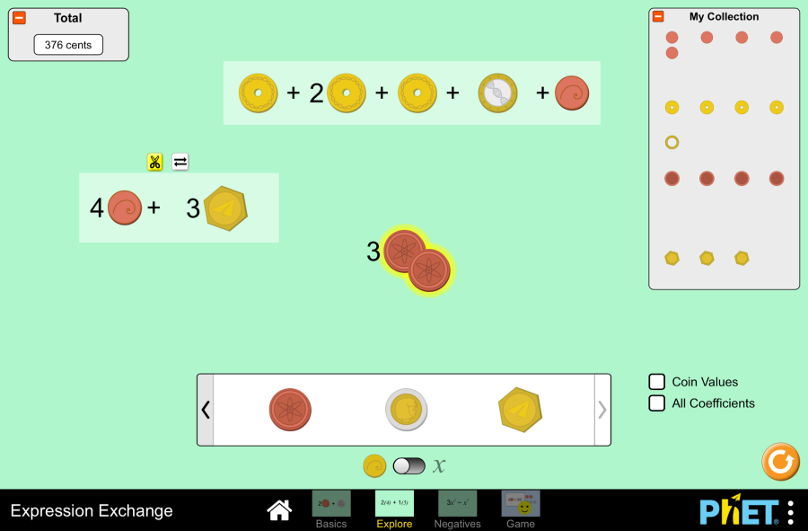
Objective: This virtual work is intended for use in math lessons in the following chapter: Virtual Experiment The virtual work “Efficient Calculations” is intended for students to learn how to make calculations with different coins and reduce expressions. Workflow: Step 1. Run the simulation. You have 4 different modes. “Basics”, “Explore”, “Negatives”, “Game”. You will work in the “Explore” and “Game” sections. Open the “Explore” section. Step 2. In the work area, you are provided with: Step 3. Pull out some coins to the work area. When you hold the coins in one row, part of the screen turns whitish, forming a sum. You can see the sum on the board, where the value of the expression is shown. Step 4. Activate the buttons to display the values ​​​​and coefficients of the coin. Step 5. Build the next expression. Build several expressions using coins. Step 6. You can replace the coin with the variables x, y, z. Step 7. Open the “Game” section. You are given 8 levels. In this lesson, you will work on the first 4 levels. Step 8. Open the first level. In the work area you are provided with: Step 9. Build expressions by looking at the expression panel given for assembly and drag them to the empty space under the expression. Step 10. After you have completed the entire expression on the board, you can move to the next level by clicking the “Next” button. Conclusion Students, working on the simulator, made calculations on the topics: generalization of expressions by similar members, coefficient.

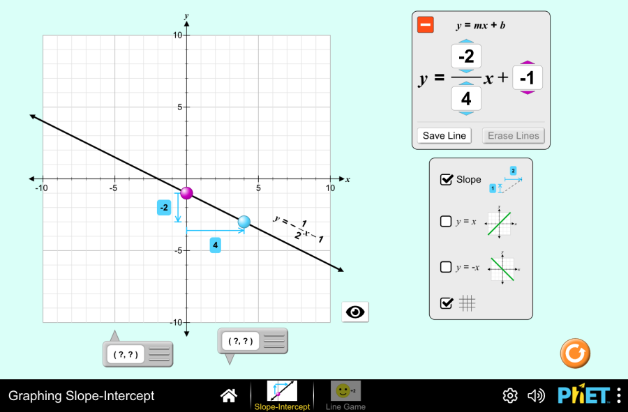
Objective: This virtual work is intended for use in algebra lessons on the following topics: Theoretical part Definition of linear function A linear function is a function that can be written in the form: The graph of a linear function is always a straight line. Graph of the function y = kx The coefficient k determines the slope of the straight line: The graph of the function y = kx always passes through the origin (point (0; 0)). Graph of the function y = kx + b Finding points of intersection of the graph with the coordinate axes The point of intersection with the Oy axis: Substitute x = 0 into the equation of the function and find the value of y. Coordinates of the intersection point: (0; b). Point of intersection with the Ox axis: Substitute y = 0 into the equation of the function and solve the equation kx + b = 0 with respect to x. Coordinates of the intersection point: (-b/k; 0). Determining the coefficients k and b from the graph Coefficient b: We find the point of intersection of the graph with the Oy axis. Its ordinate is the value of b. Coefficient k: Choose any two points A(x1; y1) and B(x2; y2) on the graph. We use the formula: k = (y2 – y1) / (x2 – x1). Virtual experiment In the Graphing Slope-Intercept simulation, students explore a line at an angle of slope. Draws a sloping line through the equation of a given graph. Predicts how changing the values in the linear equation will affect the line shown on the graph. Predicts how changing the line shown on the graph will affect the equation. Course of Work: Section 1. Slope-Intercept Part Step 1. You will be given 2 different modes, “Slope-Intercept” and “Line game”. Start the “Slope-Intercept” mode. Step 2. You are given:  Step 3. Determine the points of the graph of y = ⅔x + 1 using the tools that show the values of the points (x, y) in the graph coordinate. add buttons to show graphs of y = x and y = – x. Examine the graph. Step 4. Change the values of m, b of the function y = mx + b and study the graph.  Step 5. Examine the graph by changing the m, b values of the function y = mx + b. You can use the buttons and tools provided on the screen. Make some calculations. Section 2. Game Part Step 6. Activate the “Line Game” mode. You are given 4 levels. Select the first level. Step 7. You are given:  Step 8. You have an equation or graph in green. This is the task you must complete:   Complete and review the assigned problem.  Step 9. Complete the assignment and move on to the next level.  Conclusion The virtual lab is a valuable tool for students to learn the graphs of linear functions. The simulator has become interactive and visually useful by providing various tools for learning graphs, such as displaying points, displaying equations, and saving graphs.

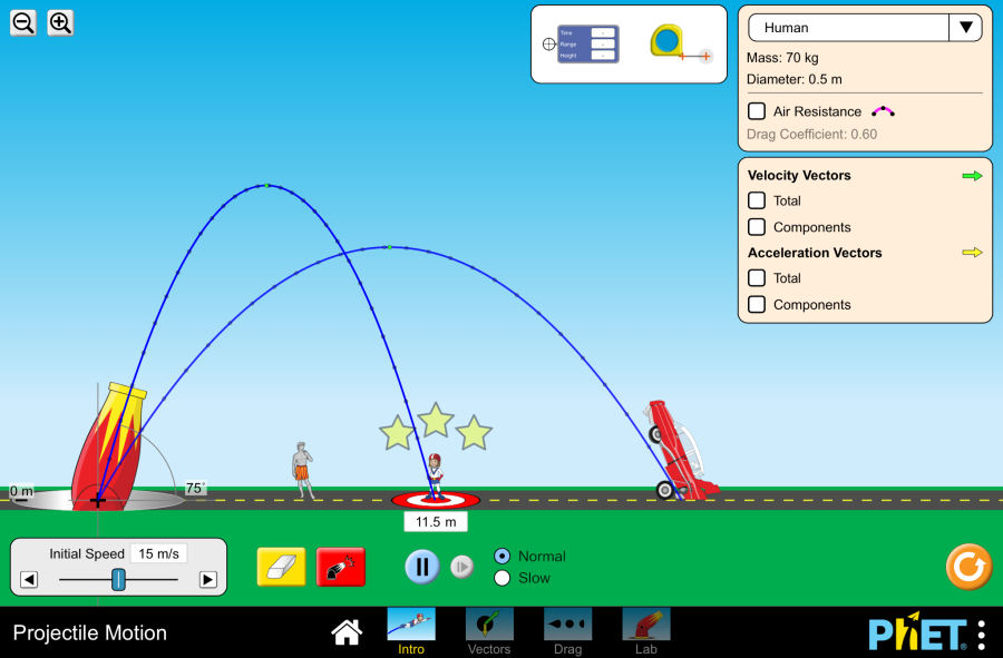
Objective: This virtual activity is designed to be used in a 9th grade geometry class. Theoretical Part The motion of a projectile is a classical problem in mechanics, often considered in a simplified model where air resistance is not taken into account. However, under realistic conditions, air resistance has a significant effect on the trajectory of the projectile, especially at high speeds and significant altitudes. Trajectory Without considering drag, the trajectory of the projectile is a parabola. Air resistance deforms this parabola, reducing the range and maximum height of lift. Vectors and Forces Velocity: A vector quantity characterizing the speed and direction of motion. Acceleration: A vector quantity that characterizes the change in velocity in magnitude and direction. Gravity: A constant force directed vertically downward. Drag force: Depends on velocity, air density, cross-sectional area, and drag coefficient. Motion in the X and Y Axes The motion of a projectile can be decomposed into two independent components: horizontal and vertical. Only the horizontal component of the initial velocity acts on the x-axis, while gravity and air resistance act on the y-axis. Virtual Experiment In Modeling Projectile Motion, students study factors that affect the trajectory of a projectile, such as angle, altitude, initial velocity, and drag. By combining their math and physics knowledge, students can perform a variety of projectile experiments. Workflow: Step 1. Start the simulation: you will be presented with 4 different modes: “Intro”, “Vectors”, “Drag” and “Lab”. In this paper you will work in the “Intro” mode. Open the “Intro” section. Step 2. In the workspace you are given: Step 3. Shoot the projectile. Object Pumpkin. Using the Explorers tools, measure time, path, height, distance. Step 4. Add air effects, velocity vectors and acceleration vectors. Use the special tool to estimate where the object will land.    Step 5. Fire and examine the projectile. Step 6. Change the initial velocity. Fire and examine the projectile. Step 7. Change the height of the projectile, the angle. Shoot and check the projectile. Step 8. Perform several experiments by changing the settings. Notice how each setting (initial height, initial angle, initial velocity) affects the trajectory of the object with and without air resistance. Step 9. The Object Data panel lists several object names: cannonball, tank shell, golf ball, baseball, soccer ball, pumpkin, human, piano, car. Select one of the objects. Snapping on the selected object changes its mass, diameter.  Step 10. Do some experiments and research by changing the settings of the selected object.  Conclusion The study has allowed a deeper understanding of the physical processes occurring during the movement of the projectile in the atmosphere. The main parameters influencing the trajectory were taken into account: initial velocity, flight angle, mass, diameter and height. The results obtained can be used to solve various practical problems.

Objective: This virtual activity is designed for use in 7th grade algebra lessons on the following chapter: Theoretical Part Imagine a machine that transforms some numbers into other numbers. You give it one number as an input and it gives you another number as an output. This machine is an example of a function! A function is a rule that matches every number from one set with only one number from another set. How do you write a function? A function is usually written as a formula: y = f(x) Here: For example: Function y = 2x + 1. If we replace x with the number 3, we get y = 2 * 3 + 1 = 7. The function has matched the number 7 with the number 3. Examples of functions from life Virtual Experiment This virtual activity introduces students to the concept of function. In the simulation, they will calculate and investigate a hidden function based on the given arguments and the value of the function.  Procedure: Step 1. Launch the simulation. You have 4 different modes. “Patterns”, “Numbers”, “Equations” and “Mystery”. In this paper you will work in the “Mystery” section. Open “Mystery”. Step 2. In the workspace you will be given: Step 3. Enter several arguments into the function machine. Examine the results, try to find the hidden function.  Step 4. Test your guess by clicking the “show hidden function” button hidden on the function engine.  Step 5. Refresh the hidden function. Enter the arguments and try to find the hidden function. Check your guess by clicking the “Show hidden function” button. Step 6. Do some research on the function machine by increasing the number of operations by 2 and entering the arguments.  Step 7. Check your guess by clicking the “Show hidden function” button hidden on the function machine.  Step 8. Do some research by using the buttons presented on the screen on the function machine. Conclusion Students were introduced to the concept of function in a virtual activity. The function engine was an effective tool for visualizing and analyzing mathematical relationships. The variety of controls (panels, graphs, tables) gave students the flexibility to explore the function from different angles.