Virtual math

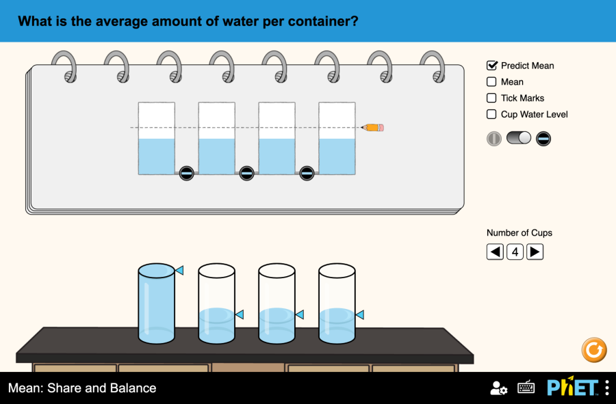
Objective: This virtual activity is designed for use in geometry lessons on the following topic: Theoretical part Arithmetic mean The arithmetic mean is a number that shows the average of all the numbers in a group. To find the arithmetic mean, you need to add up all the numbers and divide the resulting sum by the number of those numbers. Formula: Average = (Sum of all values) / (Number of values) Example: Suppose we have a data set of 5 measurements of people’s height: 170 cm, 175 cm, 180 cm, 185 cm, 190 cm. Average: (170 + 175 + 180 + 185 + 185 + 190) / 5 = 180 cm. Virtual Experiment Modeling “mean fraction and equilibrium” allows students to understand mean in a variety of contexts. Students observe how gravity balances the height of water in two-dimensional beakers when the valves are opened. The flattened height is the average level of water in the beakers. Procedure: Step 1. Launch the simulation. In the workspace you will find Step 2. Activate the Predicted Average, Marks and Water Level buttons. Looking at the marks in the beaker, if it balances the water in the beaker, guess where the water level reaches the beaker by moving the knob there. Step 3. Press the middle button. Click “Restore Balance”. Compare the actual average water level with the estimated average water level.  Step 4. Press the “Restart” button. Increase the number of jars as desired.  Step 5. Repeat the process for 2 cups. Step 6. Experiment by changing the number of cups to your liking.  Conclusion Students were introduced to the concept of average through this virtual activity. They performed different manipulations of different levels of water in a beaker and balanced the water.

Objective: This virtual activity is designed to be used in math lessons in the next chapter: Theoretical part A ratio is a comparison of two quantities. It shows how many times one quantity is greater or less than the other. A ratio is written as a fraction or with a colon. For example, the ratio of the number of apples to the number of pears is 3:5, which means that there are 1.67 times fewer apples than pears. Proportion is the equality of two ratios. It is written as two fractions separated by an equal sign. For example, 3/5 = 6/10 is a proportion. Proportions are widely used to solve various problems related to the proportional dependence of quantities. Basic properties of proportions: Virtual experiment In the Ratio and Proportions game, students explore the concepts of ratio and proportional reasoning by changing hand positions and supporting ratios with movement to find complex relationships. Move your hands to find a complex ratio and try to maintain the ratio by moving your hands together. Workflow: Step 1. You have 2 different modes, “Discover” and “Create”. Open the “Discover” section.  Step 2. Start the simulation. In the workspace you will see: Step 3. Press the “Display with line scale” button. You will see that the pointer is in row 2 and 4 and the screen is green. Step 4. If you change the position of one of the hands, you will notice that the screen color changes. This is because the ratio between the two numbers is broken. The ratio between the hands is 2 multiples of 2. Step 5. Place one hand on the number 3. Place the value of the other hand on the number 6, which is 2 multiples of 2. The ratio of 2 is maintained and the screen turns green. Step 6. Construct several proportions that maintain this ratio of numbers. For example, 3.5 and 7; 5 and 10, and so on.  Step 7. Select Challenge 2. Here you construct a ratio of 3 times the numbers.  For example, 1 and 3; 2 and 6, etc. Step 8. Select Challenge-3. This is where you create a relationship to 1.33 times the numbers.  For example, 2 and 2.66; 6 and 8, etc. Step 9. Open the Create section. In the workspace you will see: Step 10. Press the button “Display with line scale”. Choose the size of the line. Step 11. Move your hand over the specified multiple. If it is correct, the screen will turn green.  Step 12. Activate the lock button. Create different proportions of numbers by moving your hands. Step 13. Give other types of proportional relationships and do experiments. Conclusion This virtual activity can help students master the topic of proportions. Creates different relationships, and realizes the topic more deeply.

Objective: This virtual work is intended for use in 6th grade mathematics classes. Theoretical Part Imagine a machine that transforms some numbers into other numbers. You give it one number as an input and it gives you another number as an output. This machine is an example of a function! A function is a rule that matches every number from one set with only one number from another set. How do you write a function? A function is usually written as a formula: y = f(x) Here: For example: Function y = 2x + 1. If we replace x with the number 3, we get y = 2 * 3 + 1 = 7. The function has matched the number 7 with the number 3. Examples of functions from life Virtual Experiment This virtual activity introduces students to the concept of a function. The simulator is not designed to calculate with numbers, but with images as arguments; a function is designed to transform these images. On the Expression screen, students explore different functions and make predictions. They can play detective to find hidden functions on the puzzle screen. Workflow: Step 1. Start the simulation. There are 2 different modes. “Patterns” and “Mystery”. Open the “Patterns” section. Step 2. In the workspace you are provided with: Step 3. Place an operation on the function machine. There are 12 different operations, choose one. Step 4. Paste the image from the argument panel into the machine. How did the function transform the image?  Step 5. Insert some more pictures into the machine and study the function.  Step 6. Add three operations to the machine. Add three different operations to the machine.  Step 7. Paste an image from the argument table into the machine. How did the function transform the picture?  Step 8. After each operation performed on the input number in the function machine, activate the button that displays the value of the expression. Run a few more images and examine how the image changes after each operation. Step 9. Open “Mystery”. In the workspace provided: Step 10. Enter several images into the function engine. Examine the results, try to find the hidden function.  Step 11. Test your assumption by clicking on the hidden “show function” button on the function machine.  Step 12. Do a little research by increasing the number of operations on the function machine and inserting images.  Conclusion Students have become familiar with the concept of function in the virtual lab. They have seen that its role in mathematics is important. This work serves as an introduction to the topic of function in high school. They realized that function is not just a formula, but a way of describing the relationship between quantities in the world around us.

Objective: This virtual activity is designed for use in geometry lessons on the following topic: Grade 9. “Sum of Vectors”. Theoretical Part A vector is a directed line segment that is characterized by The Vector Addition Operation Vector addition is a geometric operation to find a new vector by adding two or more vectors. Properties of vector addition Virtual Experiment In this virtual activity, students explore vectors in one-dimensional space and investigate how vectors add up. By placing vectors in Cartesian coordinates and examining the magnitude, angle, and components of each vector. They can use different representations to accomplish different tasks.  Workflow: Step 1. Start the simulation: You will be presented with 4 different modes: “Explore 1D”, “Explore 2D”, “Lab” and “Equations”. In this paper you will work in the first 2 modes. Open the “Explore 1D” section.  “Explore 1D” Section One-dimensional space: This is a line that extends infinitely in two opposite directions. It is described by a single coordinate (for example, the X axis). Step 2. In the workspace provided to you: Step 3. Place the vector a on the coordinate plane. The board above shows the vector data. Step 4. Execute the buttons Sum, Values. Examine the vector  a. |a| -values, |s| -sum. Step 5. Place vector b in the plane. |b| – indicates the length of vector b, |s| -sum indicates the sum value of vectors a and b. Since |s| is the sum value, it does not depend on the location of vectors a and b in the plane, so the value of |s| does not change. Step 6.Place the vector c in the plane. |c| is the length of the vector c, |s| is the sum value of the vectors sum a, b, c. Step 7. You can move the coordinate plane from horizontal to vertical and perform calculations for vectors d, e, f. “Explore 2D” Section Two-dimensional space: used to graph functions and equations. The X-axis is horizontal and the Y-axis is vertical. All the shapes we learn in school geometry (triangles, squares, circles, etc.) are two-dimensional. Step 8. In the workspace, you are given Step 9. Place the vector a on the coordinate plane. The table above shows the data of the vector. |a| – length of the vector, – angle, ax, ay – length along the x,y axes.  Step 10. Activate the Sum, Value, Angle buttons. Explore the different layouts of the vector a for ax, ay by clicking each button on the Component panel.  Step 11. Place vector b in the plane. Examine the value of the sum |s|.  Step 12. Place vector c in the plane. Examine the value of the sum |s|.  Step 13. Choose the type of vector by angle and perform calculations for vectors d, e, f.  Conclusion By working on this simulation, students became more familiar with the concept of vectors and sharpened their skills in adding vectors. Verified that the sum of vectors depends on their dimensions and angles. Studied the arrangement of vectors in one- and two-dimensional space and visualized the arrangement of objects in space.

Objective: This virtual activity is designed for use in geometry lessons on the following topics: Theoretical part A vector is a directed line segment characterized by Multiplying a vector by a scalar Multiplying a vector by a scalar changes the length of the vector. If the scalar is positive, the direction of the vector is preserved; if it is negative, the direction is reversed. Addition and Subtraction of Vectors A line equation is a mathematical expression that defines all the points that lie on a given line in the plane. One of the most common ways to write the equation of a line is the general equation: Ax + B + C = 0 where A, B, and C are some constant numbers, and at least one of A or B is not zero. The geometric significance of the coefficients Virtual Experiment In the “Vector Addition: Equations” virtual activity, students experiment with vector equations and compare vector sums and differences. Students learn about scalar multiplication by performing calculations with vectors and changing the coefficients in an equation. Workflow: Step 1. Launch the simulation. In the workspace provided: Step 2. Explore the information of the vector data panel by clicking vectors a, b, c.  Step 3. Activate the “Values” and “Angle” buttons. Explore the different layouts of the vectors by clicking on each button in the Components panel. Step 4. Perform a vector calculation using the equation a+b=c. Change the coefficients of the vectors a and b and solve the problems.  Step 5. Modify the vectors a and b by changing the values ax, ay for the vector a, bx, by for the vector b from the vector coordinates panel. Since a+b=c, the vector c is changed automatically.  Step 6. Click the Reload button. Select the equation a-b=c.  Step 7. Repeat the operations created for the equation a+b=c and examine the vectors.  Step 8. Click the Reload button. Select the equation a+b+c=0. Step 9. Repeat the operations created for the equation a+b=c and examine the vectors.  Step 10. You can select the vector type by angle and perform calculations for the vectors d, e, f.  Conclusion Students learned more about the concept of a vector by working on this simulation. They studied and compared the changes that occur when a vector is multiplied by a scalar, and the results of adding and subtracting vectors. Mastered techniques for adding vectors using the parallelogram rule and the triangle rule.

Objective: This virtual activity is designed to be used in the math lessons in the next chapter: Theoretical part 1. Definition and representation Examples: 2. Comparing positive and negative numbers on the number axis 3. Operations on positive and negative numbers Addition: Subtraction: 4. Modulus of a number The modulus of a number is its absolute value, i.e., its distance from zero. The modulus of a number is always a non-negative number. Notation: The modulus of a is written as |a|. Examples: |5| = 5, |-3| = 3, |0| = 0. Virtual Experiment The “Number Line: Operations” simulator is based on integers, which allows you to perform operations on integers.  Workflow: Step 1. Start the simulation: you will be offered 4 different modes: “Chips”, “Net Worth”, “Operations” and “Generic”. Open the “Chips” section.  Section 1. Calculating Coins Students can play by adding and subtracting integers using the coin pattern. Step 2. In the work area, you will find Step 3. Put the coins into the bag with the green strap. You can put in up to 15 coins. Calculate your income by adding the coins. Step 4. Put the coins into the bag with the red ribbon. You can put up to 15 kopecks. Calculate your expenses by adding the coins. If your income is equal to your expenses, your score is 0. Show negative numbers by coordinates if you have more expenses. Shows positive numbers by coordinates if your income is higher.  Part 2. Status Screen Students can use real-world examples to reinforce their understanding of integer operations. Step 5. Open the Net Worth section. In the workspace, you will see: Step 6.Here you can perform various operations and calculations on your assets and liabilities. Section 3. Operations Screen  Students can set an initial net worth and then perform operations on it. In this section, you will only work with hundredths of a percent. For example, 100 200 300. Step 7. Open the Operations Section. In the work area you will find Step 8. Set the initial net cost. Step 9. Select any hundred on the hundredths board and add it. Step 10. Go to the second hundred board and mark and subtract some hundreds. In this way, try different operations and make calculations. Section 4. Generic Screen The Generic screen provides flexibility in modeling operations with integers, working with numbers up to 100, and using the number line to reinforce abstract understanding of operations. Step 11. Open the Generic Section. The work area provides you with Step 12. Mark the initial number by moving the blue point.  Step 13. Mark and add any number in the number field. Step 14. Go to the second number board and mark and subtract any number. In this way, try different operations and perform calculations. Step 15. Mark two coordinate axes for the work area. Perform two separate calculations on each axis. Compare the axes. Conclusion On the horizontal number line, the addition and subtraction of whole numbers has been pictorially calculated in terms of the order of the numbers. Recognized and created equivalence classes of whole number sums and differences. Verified that the sum of a number and its additive inverse is 0.

Objective: This virtual activity is designed to be used in the math lessons in the next chapter: Theoretical part 1. Definition and representation Examples: 2. Comparing positive and negative numbers on the number axis 3. Modulus of a number The modulus of a number is its absolute value, i.e., its distance from zero. The modulus of a number is always a non-negative number. Notation: The modulus of a is written as |a|. Examples: |5| = 5, |-3| = 3, |0| = 0. Virtual Experiment In the “number line: integers” simulation, students can explore the many contexts in which integers can be compared to integers on a number line. After students explore height, bank accounts, and temperature, they can make generalizations about comparing integers and determine absolute value.  On the Explore screen, students can compare integers in different contexts.  On the Generic screen, students can compare whole numbers on different scales and begin to define absolute value in a general way. Workflow: Step 1. Start the simulation: You will be given 2 different modes, “Explore” and “Generic”. Open the “Explore” section.  Step 2. In the work area you are given: Step 3. Position the person on the plane. Start the absolute value button. Explore the data from the coordinate axis associated with altitude, moving the person across the water, sky, and mountains.  Step 4. Place the bird and fish on the plane. Explore data from the comparison panel by moving 3 objects to different locations on the plane.  Step 5.Open the section with the piggy bank image. You are given: Step 6. Click the absolute value. Do some operations and make a comparison by picking up and licking a coin on the piggy bank. Step 7. Add 2 piggy banks to the coordinate axis that shows the balance. Do a comparison by counting the coins in these 2 piggy banks.  Step 8. Open the section showing the thermometer. You are given: Step 9. Change the unit of temperature measurement to degrees Celsius. Place the thermometer on the map and measure temperatures in different parts of the Earth.  Step 10. Place the remaining 2 thermometers on the map and make a comparison by examining the temperature changes in each part of the world.  Step 11. Change the month from January to another month and examine and compare the temperature changes.  Step 12. Open the Generic section. In the workspace you are provided with: Step 13. Activate the data display buttons on the coordinate axis. Explore the data by moving the point on the coordinate axis.  Step 14. Add 2 more points to the coordinate axis and make a comparison by moving them. Step 15. Change the length and position of the coordinate axis and make some more comparisons.  Conclusion The simulator can be an aid in mastering the concept of absolute value so that students can familiarize themselves with negative numbers. Describing the position of a point in a number line with respect to another number, describing the position of a number line with respect to the opposite side of a point, they made sure that the negative number was smaller than the positive number each time. 

Objective: This virtual activity is designed to be used in the math lessons in the next chapter: Theoretical part 1. Definition and representation Examples: 2. Comparing positive and negative numbers on the number axis 3. Operations on positive and negative numbers Addition: Subtraction: Multiplication: Division: 4. Modulus of a number The modulus of a number is its absolute value, i.e., its distance from zero. The modulus of a number is always a non-negative number. Notation: The modulus of a is written as |a|. Examples: |5| = 5, |-3| = 3, |0| = 0. Virtual Experiment The Number Line: Modeling Distance simulation teaches students to subtract in different contexts, identify patterns, and generalize about how to interpret subtraction as distance. The Explore screen allows students to explore subtraction with two objects and determine whether the distance between them is taken into account in subtraction. The Generic screen provides flexibility to reason about subtraction in any context or out of context, and generalizes the concept of subtraction as the distance between two integers on a number line.  Workflow: Step 1. Start the simulation: You will be given 2 different modes, “Explore” and “Generic”. Open the “Explore” section.  Step 2. In the workspace you are provided with Step 3. Position the house and person on the plane. Examine the coordinate axis data. What is the absolute value?  Step 4. Click the Simple Value button. How has the data changed in the Calculation Panel?  Step 5. Click the Move Bodies button. Examine the data on the coordinate axis and in the Calculation Panel.  Step 6. Click the Absolute Value button. Examine the changes in the calculations again.  Step 7. Change the distance between the house and the person. Perform the study by repeating the above steps. Step 8. Open the second case of the calculation. Here you will study the temperature difference.  Step 9. Place the thermometers on a plane representing the seasons. Just as you would study the distance between a house and a person, you will study between temperatures.  Step 10. Open a third case. Here you are investigating the vertical distance between a bird and a fish. Step 11. Place the bird in the sky and the fish in the water. Research between them as you would research the distance between a house and a person.  Step 12. open the Generic section. In the workspace you are provided with: Step 13. Place two points on the coordinate axis. Examine the data on the Coordinate Axis and on the Calculation Panel. Step 14. Explore the distances between the bodies by performing different point calculations.  Conclusion Students have explored the relationship between horizontal and vertical number lines and the coordinate plane. This simulation provides real-life situations that set the stage for applying the knowledge in real life. Absolute value, application of operations to rational numbers can serve as a tool for mastering the topics.

Objective: This virtual activity is designed to be used in math lessons in the next chapter: Theoretical part Multiplication Operation Imagine you are a baker and you want to bake lots of delicious pies. How many pies will you get if you use 2 cups of flour for each pie? That’s where multiplication comes to our rescue! Multiplication is the addition of identical groups. In our case: 1 pie = 2 cups of flour 2 pies = 2 cups of flour + 2 cups of flour = 4 cups of flour. 3 pies = 2 cups flour + 2 cups flour + 2 cups flour + 2 cups flour = 6 cups flour Let’s write it down like this: 2 x 3 = 6, where: 2 is the multiplier (what we are multiplying) – the amount of flour for 1 pie 3 is the multiplier (how many times we multiply) – the number of pies 6 is the product (the result of multiplication) – the total amount of flour. Division operation The more pies we bake, the more flour we use! Now let’s imagine that you have 8 delicious apples and you want to put them equally into 2 baskets. How many apples will be in each basket? Division will help us with that. Division is dividing a number into equal groups. In our case: 8 apples / 2 = 4 apples in each basket We write it like this: 8 : 2 = 4, where: 8 is the divisor (what we are dividing) – the total number of apples 2 is the divisor (how many groups we divide into) – the number of baskets 4 is the quotient (the result of division) – the number of apples in each basket. Let’s write it like this: 8 : 2 = 4, where: 8 is the divisor (what we are dividing) – the total number of apples 2 is the divisor (how many groups we divide into) – the number of baskets 4 is the quotient (the result of division) – the number of apples in each basket. The more apples, the more baskets with the same number of apples you get! Multiplication and division are like two sides of the same coin: Virtual experiment The “multiplication” simulation is an aid for students to familiarize themselves with the multiplication table. The screen introduces the multiplication operation in the form of the Pythagoras table. By manipulating the numbers, he gets the results of multiplication. Course of Work: Step 1. Start the simulation: You will be offered 3 different modes: “Multiply”, “Factor” and “Divide”. Open the “Multiply” section.  Part 1. “Multiply”. Step 2. You are given 3 levels: Level 1 performs multiplication of numbers 1-6, Level 2 1-9, and Level 3 1-12. Choose Level 1. In the workspace, you are given: Step 3. The Pythagoras table displays an expression that is colored and multiplied below the table. Write the value of the multiplication in the box where you write the result of the multiplication. Step 4. Click the “Check” button. If the result is correct, the expression of the next product is given. If there is an error, the “try again” button will appear. If there is an error, click the same button and write the result of the product from the beginning. Step 5. You can complete all the level 1 productions and go to the next level, or you can complete some more level 1 productions from the beginning.  Part 2. “Factor”. Step 6. Open the “Factor” section. There are 3 levels: Level 1 does multiplication of numbers 1-6, Level 2 does multiplication of numbers 1-9, and Level 3 does multiplication of numbers 1-12. Step 7. You are given in the work area: Step 8. The expression below the table gives the result of the product. In the Pythagoras table, mark the two numbers you need to multiply. Step 9. If the result is correct, the expression for the next product is given. If there is an error, a “try again” button appears. If there is an error, press the same button and write the result of the product from the beginning.  Step 10. You can complete all level 1 pieces and go to the next step, or you can complete some more level 1 pieces from the beginning. Part 3. “Divide”.  Step 11. Open the “Divide” section. There are 3 levels: Level 1 does multiplication of numbers 1-6, Level 2 does multiplication of numbers 1-9, and Level 3 does multiplication of numbers 1-12. The work area is similar to the “Multiply” section. Step 12. The expression below the table gives one of the multiplication numbers and the result of the product. Find the second number to multiply. Check the second number by marking it on the Calculator bar. Step 13. If the result is correct, the expression of the next product is given. In case of an error, the “Try again” button will appear. If there is an error, press the same button and write the result of the product from the beginning.   Step 14. You can finish all level 1 productions and go to the next step, or you can do some more level 1 productions from the beginning. Conclusion Students will learn how to multiply using the Pythagorean table through this virtual activity. This is interesting for students because they work with the multiplication operation visually and it makes it easier to memorize the multiplication table.

Objective: This virtual activity is designed to be used in the math lessons in the next chapter: Theory A derivative is a mathematical function that shows the rate of change of another function. Studying the graph of the derivative provides valuable information about the behavior of the original function. 1. The relationship between the graphs of f(x) and f'(x) The points of intersection with the x-axis: The x-coordinates of the points of intersection of the graph of the derivative with the x-axis are the points of extremum (maximum or minimum) of the original function. Intervals of monotonicity: If f'(x) > 0 on the interval (a, b), then f(x) is increasing on this interval. If f'(x) < 0 on the interval (a, b), then f(x) is decreasing on that interval. Local maxima and minima: A point x0 is a maximum point of f(x) if f'(x0) > 0 and then f'(x) < 0. A point x0 is the point of minimum of f(x) if f'(x0) < 0 and then f'(x) > 0. Asymptotes: The horizontal asymptote y = L if limx → ±∞ f(x) = L. The vertical asymptote x = a if limx → a f(x) = ±∞. 2. Algorithm to study the graph of the derivative Virtual Experiment The Exploring the Graph of a Function Using the Derivative virtual activity allows students to explore and determine relationships between the graphs of a function and its derivative. On the derivative screen, students can change the function and view the graph of its derivative. Course of work: Step 1. Start the simulation: You will be presented with 4 different modes: “Derivative”, “Integral”, “Advanced” and “Lab”. In this work, you will be working in the “Derivative” section. Open the “Derivative” section. Step 2. In the workspace provided to you: Step 3. Click the Planes grid display button. Step 4. Draw the graph of the function f(x). Draw the graph by raising or lowering the blue line along the OX axis. If you raise the line, it is the function – cos(x), if you lower it, it is sin(x). You will automatically have a graph of the derivative in the lower plane. If f(x)=cos(x), then f'(x)=sin(x). If f(x)=sin(x), then f'(x)=cos(x). Step 5. Click view Tangent graph. A discontinuous line with a red straight line and a round head appears on the screen. Explore the movement of the tangent graph by moving the wheel over the graph of the function. You can also see that the tangent has a different value in each part of the graph in the panel that appears on the left.  Step 6. Delete the graph on the plane by clicking the eraser. Change the volume of the wave.  Step 7. Draw the graph by raising or lowering the blue line along the OX axis. Examine the graphs of the functions f(x) and f'(x) and the movement of the tangent along the graph. If the graph of the derivative is not displayed completely in the plane, you can click the “-” button and zoom out. Step 8. Delete the graph on the plane by clicking on the eraser. Select the second type of graph. The function f(x) is a complex function. Draw the graph by moving the blue line up or down.  Step 9. Examine the graphs of the functions f(x) and f'(x) and the movement of the tangent on the graph. Step 10. Delete the graph in the plane by clicking on the eraser. Select the third type of graph. Here f(x)=±kx. Draw the graph by raising or lowering the blue line along the OX axis.  Step 11. You have f'(x) = ±k. Study the graphs of the functions f(x) and f'(x) and the movement of the tangent along the graph.  Step 12. Delete the graph in the plane by clicking on the eraser. Select the type of the fourth graph. Here f(x)=±k. Draw the graph by raising or lowering the blue line along the OX axis.  Step 13. You have f'(x)=0. Study the graphs of the functions f(x) and f'(x) and the movement of the tangent along the graph.  Conclusion Through this virtual activity, students have studied the graphs of derivative functions using graphs of given functions. They have also studied the tangent, one of the most important elements of the graph of a function. Since the use of the derivative is an early, important topic in mathematical analysis, this simulation can be very useful for students.