Virtual math

Objective: This virtual activity is designed to be used in math lessons in the next chapter: Theoretical part 1. Definition: A linear equation with one variable is an equation of the formaah+b=0, where: a and b are arbitrary numbers (coefficients of the equation), wherea0. x is the unknown variable. 2. Examples: 3. Solving a linear equation: Goal: To find all values of the variable x at which the equation becomes true. Algorithm: Example: 3x – 5 = 0 3x = 5 x = 5/3 Answer: x = 5/3. Virtual Experiment On the equation screen, students can interpret, compare, and translate multiple representations of an algebraic function. It can predict the output of a function on given inputs and create a new function. Workflow: Step 1. Start the simulation: you will be presented with 4 different modes: “Patterns”, “Numbers”, “Equations” and “Mystery”. You will work on this experiment in the “Equations” section. Open the “Equations” section. Step 2 You are given:  Step 3. Open the tables on the function machine. Step 4. Place an arithmetic operation on the function machine. You can change the numbers with an interval from -3 to +3. You can use addition, subtraction, multiplication and division operations.  Step 5. Enter the incoming number into the function machine. The input panel shows the numbers (-5; 7) and the variable x. Step 6. You can see the number of inputs, function value, graph and equation in the tables. The function value panel shows the value of the expression. Step 7. Place more different arithmetic operations on the function machine. You can place up to three techniques there. Step 8. Put the input number into the function machine. Examine the function data.  Step 9. Activate the button indicating the value of the expression.  Enter the input number into the machine. After the first operation, the value of the expression is displayed.  Step 10. To perform the next operation, you pass the expression value to the next operation by holding down the left side of the mouse. Step 11. Change the data as you see fit and create different expressions. You can use the input numbers panel, operations. Conclusion For students, working with a given function machine in virtual work is an easy way to explore functions and their effect on input data. Following the steps in sequence allowed them to experiment with different arithmetic operations and input numbers, and to observe changes in function values and equations.

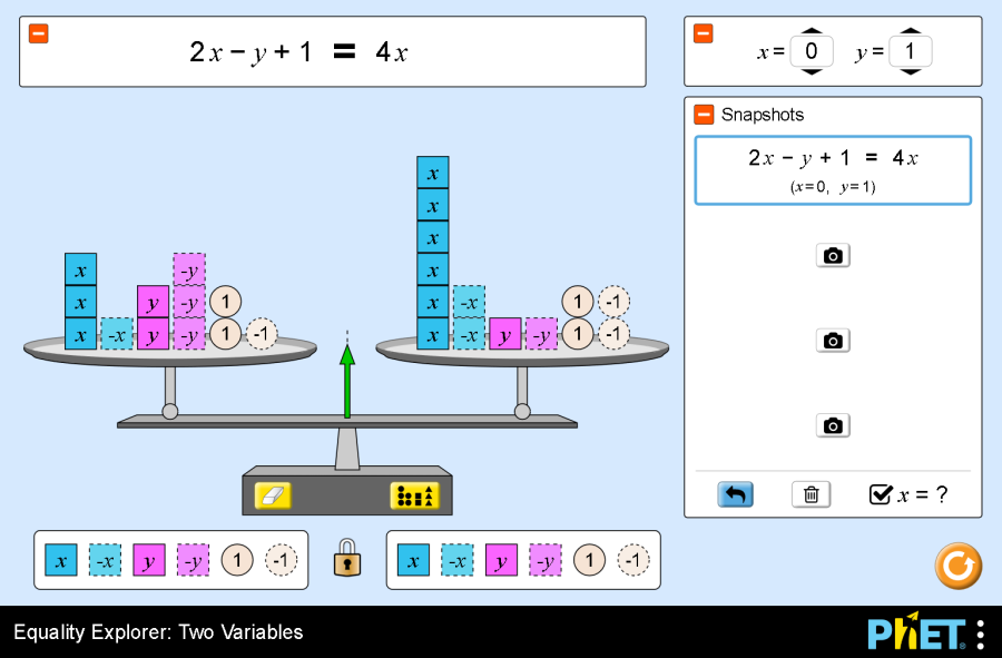
Objective: This virtual activity is designed to be used in math lessons in the next chapter: Theoretical part A linear equation with two variables x and y (with two unknowns x and y) is an equation of the form a*x+b+y+c=0, where a,b,c are numbers, and a and b are not equal to 0 at the same time. For example, -2x+7y=0; 12x-11y+5=0 are linear equations with two variables. Since in such equations there are two variables, so the solution to equations with two variables is not one but two numbers, which are usually written in parentheses, and the number that we substitute into the equation instead of x, we write in the first place, and y – in the second place: (x, y). The solution of an equation with two variables a*x+b+y+c=0 is such a pair of numbers, when substituting which instead of x and y in the equation, the correct numerical equality is obtained. For example, the pair of numbers (0,5;1) is a solution to the equation with two variables 12x-11y+5=0. To solve a linear equation with two variables is to find the set of solutions.  If a pair of numbers is a solution to an equation with two variables, the pair is also said to satisfy the equation. Equations with two variables are called equivalent if all the solutions of one equation are equal to the solutions of the other equation. Virtual experiment The “Equality Explorer: Two Variables” simulation allows students to explore the conditions that result in equality and inequality when there are two variables present. Students can build a system of equations and develop a meaningful understanding of a system of equations. Workflow: Step 1. You are given:  Step 2. Generate an equation in x =1, y=1 values. You can use the button that adjusts the expressions over the weights. Step 3. Click the camera button and save to the image panel. Step 4. Change the value of x and make the equation. If necessary, you can use the eraser and button to adjust the expressions over the weights. Save to the image panel. Step 5. Change the x and y values and make the equation. You can click the lock button and express both sides of the equation with the same numbers. Save in the image panel. Step 6. Compose the equations by assigning different values to the x and y variables. Fill in the image panel. Conclusion Performing the virtual work “Equality Explorer: Two Variables” allowed students to deepen their knowledge of linear equations with two variables and learn how to use them to solve practical problems. The fact that the variable has a different value by balancing it on weights makes it easier for students to visualize and learn how to make different equations.

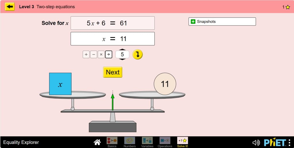
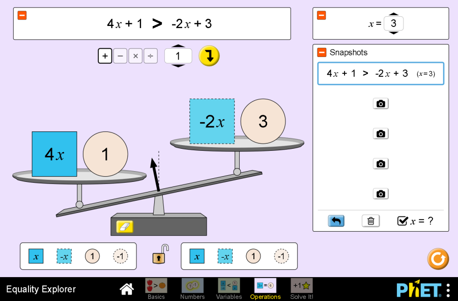
Objective: This virtual activity is designed for use in math lessons on the following topics: Theoretical part Complex equations are equations that contain two or more arithmetic operations. The number that converts it to a correct equality when you put a letter in an equation is called the solution to the equation or the root. A variable is a quantity that can take on different values. Expressions with several variables can also be simplified and then find the values at given letter values. Transformations of expressions that result in a simpler expression are called simplifying expressions. For example:  x + x + x + x + x  “4 times x” can be written shorter (simplify): 4 ∙ x or 4x.  The multiplication sign is often not written in such cases. x + x + x + x + x = 4x If a transformation can be performed on the left or right side of an equation, simplify the expression first and then solve the equation. Consider how you solved the equation.  5x + 2x = 49  The left side of the equation can be simplified. Let’s do this.  7x = 49  Now let’s solve the simple equation by the rule of finding the unknown multiplier. x = 49:7  x = 7  Verification.  5 ∙ 7 + 2 ∙ 7 = 49  35 + 14 = 49  49 = 49 Virtual experiment The “Equation” simulation allows students to explore the concept of equation, inequalities, and variables. On the “Variables” screen, students explore how different values of a variable affect the state of equality. On the “Calculations” screen, students can construct an inequality or equation and apply universal operations to find out what happens to each term and learn how to undo the operation. Progression: Part 1. Variables Step 1: Start the simulation: you will be presented with 5 different modes: ‘Basics’, ‘Numbers’, ‘Variables’, ‘Operations’ and ‘Solve it’. You will work on this experiment in the “Variables”, “Operations” sections. Open the “Variables” section. Step 2. You are given:  Step 3. Generate the equation in the value of x =1. If necessary, you can use the eraser and button to adjust the items above the scales. Step 4. Click the camera button and save the equation in the image panel. Step 5. Change the value of x and make the equation. You can press the lock button and express both sides of the equation with the same numbers. Save in the image panel. Step 6. Compose the equations by assigning a different value to the variable x. Complete the image panel. Part 2. Calculations  Step 7. Open the “operations” section. You are given:  Step 8. Construct the first equation: x =1. You can construct the equation using the variables and numbers located at the bottom. You can use the operations panel above. In the operations panel, you can create expressions with numbers from 1 to 10 in the operations ( + ), ( – ), variables 1x-10x, numbers from 1 to 10 in the operations ( * ), ( / ). Click the camera button and save in the image panel. Step 9. Change the value of x and make an equation. Save to the image panel. Step 10. Compose equations by assigning a different value to the variable x. You can use all of the tools in the workspace when composing an equation. Fill in the image panel. Section 3. Solving an equation Step 11. Open the “Solve it” section. You are given levels of the equation:  Step 12. Level 1: Discover one-step equations. In the work area you are provided with: Step 13. Equation to be solved solve the equation using the operations board with the given board. As you solve the equation, the value of x should remain on one side of the scale and the value of x should remain on the other side of the scale. If the equation is solved correctly, the “next” button will appear.  Step 14. Click “next” and move on to the next equation. Solve the given equation. Try solving more than one equation. Step 15. Go to other levels. Solve the equations. Conclusion The virtual “equation” simulator allowed students to gain a deeper understanding of the topic of equations. The equations that the students have learned to solve so far entered a complex form in this activity and helped them to sharpen their knowledge. The fact that the variable has a different value by balancing it on a scale makes it easier for students to visualize and learn how to make different equations.

Objective: This virtual activity is designed to be used in math lessons on the following topics: Theoretical part Compound equations are equations that contain two or more arithmetic operations. A variable is a quantity that can take on different values. Expressions with several variables can also be simplified and then find the values at given letter values. Transformations of expressions that result in a simpler expression are called simplifying expressions. For example:  x + x + x + x + x  “4 times x” can be written shorter (simplify): 4 ∙ x or 4x.  The multiplication sign is often not written in such cases. x + x + x + x + x = 4x If a transformation can be performed on the left or right side of an equation, simplify the expression first and then solve the equation. Consider how you solved the equation.  5x + 2x = 49  The left side of the equation can be simplified. Let’s do this.  7x = 49  Now let’s solve the simple equation by the rule of finding the unknown multiplier. x = 49:7  x = 7  Verification.  5 ∙ 7 + 2 ∙ 7 = 49  35 + 14 = 49  49 = 49 Virtual experiment The “Equation” simulation allows students to explore the concept of equation, inequalities, and variables. On the “Variables” screen, students explore how different values of a variable affect the state of equality. On the “Calculations” screen, students can construct an inequality or equation and apply universal operations to find out what happens to each term and learn how to undo the operation. Progression: Part 1. Variables Step 1: Start the simulation: you will be presented with 5 different modes: ‘Basics’, ‘Numbers’, ‘Variables’, ‘Operations’ and ‘Solve it’. You will work on this experiment in the “Variables”, “Operations” sections. Open the “Variables” section. Step 2. You are given:  Step 3. Generate the equation in the value of x =1. If necessary, you can use the eraser and button to adjust the items above the scales. Step 4. Click the camera button and save the equation in the image panel. Step 5. Change the value of x and make the equation. You can press the lock button and express both sides of the equation with the same numbers. Save in the image panel. Step 6. Compose the equations by assigning a different value to the variable x. Complete the image panel. Part 2. Calculations  Step 7. Open the “operations” section. You are given:  Step 8. Construct the first equation: x =1. You can construct the equation using the variables and numbers located at the bottom. You can use the operations panel above. In the operations panel, you can create expressions with numbers from 1 to 10 in the operations ( + ), ( – ), variables 1x-10x, numbers from 1 to 10 in the operations ( * ), ( / ). Step 9. Click the camera button and save in the image panel. Step 10. Change the value of x and make an equation. Save to the image panel. Step 11. Compose equations by assigning a different value to the variable x. You can use all of the tools in the workspace when composing an equation. Fill in the image panel. Conclusion The virtual “equation” simulator allowed students to gain a deeper understanding of the topic of equations. The equations that the students have learned to solve so far entered a complex form in this activity and helped them to sharpen their knowledge. The fact that the variable has a different value by balancing it on a scale makes it easier for students to visualize and learn how to make different equations.

Objective: This virtual activity is designed for use in math lessons on the following topics: Theoretical part Equation is an equality with an unknown. To find the unknown is to solve the equation. The unknown is labeled with a letter. The goal of solving an equation: to find the unknown number when solving an equation. For example: x+3=7 x=4 4 is the root of the equation. You can find the root of the equation, or you can use knowledge about the relationship between addition and subtraction. The solution of the equation must be checked. Virtual experiment The simulation “Equation” allows students to explore the concept of equations, inequalities, and variables. On the “basics” screen, students can compose equations and create functional definitions of equality and inequality. Numbers on the screen students can work with numbers and create unique equations. Progression: Section 1: Basics Step 1. Start the simulation: you will be offered 4 different modes: “Basics”, “Numbers”, “Variables”, “Operations” and “Solve it”. You will work on this experiment in the “Basics”, “Numbers” sections. Open the “Basics” section. Step 2. You are given:  Step 3. Perform a reciprocal comparison by placing items one on either side of the scales.  Step 4. Construct the first equation. Step 5. Click the camera button and save to the image panel. Step 6. Make the next equation. If necessary, you can use the eraser and button to position the items on the scales correctly.  Step 7. Create multiple equations and fill the image panel. Step 8. You can create and experiment with different equations by alternating the types of sets of items. Section 2: Numbers Step 9. Open the “Numbers” section. You are given:  Step 10. Make the first equation from the numbers. You can express the number 1 by adding and taking it several times. Step 11. Click the camera button and save to the image panel. Step 12. Make the following equation. Click the lock button and try to express both sides of the equation with the same numbers. If necessary, you can use the eraser and button to adjust the items above the Scales.  Step 13. Create multiple equations and fill in the image panel. Conclusion The virtual “Equation” simulation allowed students to gain a deeper understanding of the topic of equations. The objects had different meanings and balanced them on the scales, students were comfortable with visual perception and learned how to make different equations.

Objective: This virtual activity is designed for use in math lessons on the following topics: Theoretical part Equation is an equality with an unknown. To find the unknown is to solve the equation. The unknown is labeled with a letter. The goal of solving an equation: to find the unknown number when solving an equation. For example: x+3=7 x=4 4 is the root of the equation. You can find the root of the equation, or you can use knowledge about the relationship between addition and subtraction. The solution of the equation must be checked. Virtual experiment The simulation “Equation. Basics” allows students to explore the concept of equations, inequalities, and variables. On the “basics” screen, students can compose equations and create functional definitions of equality and inequality. On the lab screen, students can change the values of objects and create unique equations. Progression: Section 1: Basics Step 1. Start the simulation: you will be given 2 different modes, “Basics” and “Lab”. Open the “Basics” section. Step 2. You are given:  Step 3. Perform a reciprocal comparison by placing items one on either side of the scales.  Step 4. Construct the first equation. Step 5. Click the camera button and save to the image panel. Step 6. Make the next equation. If necessary, you can use the eraser and button to position the items on the scales correctly.  Step 7. Click the camera button and save to the image panel. Step 8. Create multiple equations and fill in the image panel. Section 2: Lab Step 9. Open the “Lab” section. You are given:  Step 10. Make the equation by looking at the values of each item on the board and balancing things on the scales. Step 11. Click the camera button and save to the image panel. Step 12. Change the values of the things.  Step 13. Align things on the scales and make an equation.  Step 14. Click the camera button and save to the image panel. Step 15. By changing the values of the items, create multiple equations and populate the image panel. Conclusion The virtual simulation “Equation. Basics” allowed students to gain a deeper understanding of the topic of equations. The objects had different values and balanced them on scales, students were comfortable with visual perception and learned how to make different equations.

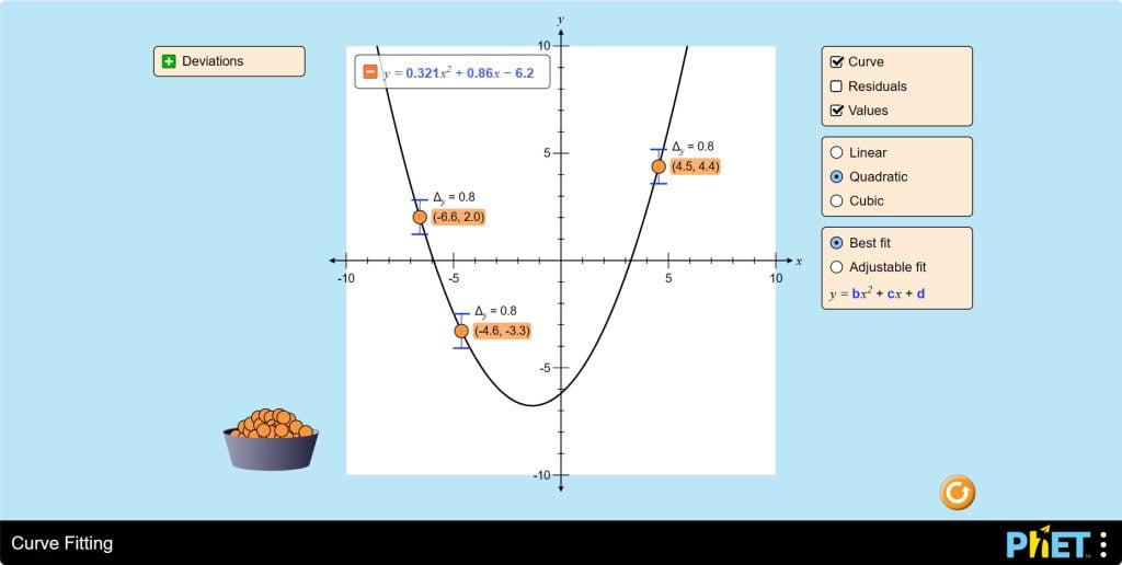
Objective: This virtual activity is designed to be used in the algebra lesson in the next chapter: Theoretical part The function 𝑦 = 𝑘𝑥 The linear function 𝑦 = 𝑘𝑥 + 𝑏 is a function whose graph is a straight line. The coefficient k determines the slope of the line. The free term 𝑏 determines the position of the line on the y-axis. Function y=ax2 The quadratic function y=ax2 is a function whose graph is a parabola. The coefficient a determines the shape of the parabola. The vertex of the parabola is at the point x=-b/2a. Function y=ax3 The cubic function y=ax3 is a function whose graph is a cubic parabola. The coefficient a determines the shape of the cubic parabola. Virtual experiment The virtual simulation is designed to familiarize and work with the functions 𝑦 = 𝑘𝑥, y=ax2, y=ax3. This allows students to easily and clearly create graphs of these functions, as well as study their properties. Workflow: Part 1. Function y=kx Step 1. Run the simulation. You are given:  Step 2. Check the function curve. You will have additional button panel: linear, quadratic, cubic equation buttons, best fit, adjustable fit.  Step 3. Since you don’t need the deviation panel in your work, you can click the “-” button and assemble it. And the use of the residuals and values buttons is not unnecessary. Step 4. Plot the 2 points on the coordinate plane. You will get the graph of the linear function y=kx+b. You can see the graphical equation at the top of the plane. Step 5. You can set the values of the points (x, y) by checking the checkbox on the coordinate button.  Step 6. Examine the change in the graph and its equation by moving the points to different locations on the plane.  Part 2. Function 𝑦 = ax2 Step 7. Change the type of equation linear to quadratic. Step 8. Place the third point in the plane. You will have a parabola corresponding to the function 𝑦 = ax2 + 𝑏𝑥 + 𝑐. Study the equation of the parabola. Step 9. Examine the change in the graph and its equation by moving the points to different locations in the plane.  Part 3. Function y=ax3 Step 10. Change the type of equation from quadratic to cubic. Step 11. Plot the fourth point in the plane. You will have a cubic parabola corresponding to the function y=ax3+bx2+cx+d. Study the equation of the cubic parabola. Step 12. Study the change in the graph and its equation by moving the points to different locations in the plane. Conclusion The virtual work described the process of graphing the linear function y=kx+b in the first section, the quadratic function 𝑦 = ax2 + 𝑏𝑥 + 𝑐 in the second section, and the cubic function y=ax3+bx2+cx+d in the third section. This simulation allowed students to extend their knowledge of the topic of function and the graph of a function by visualizing the effects of the location of points on the graph and equation in the plane.

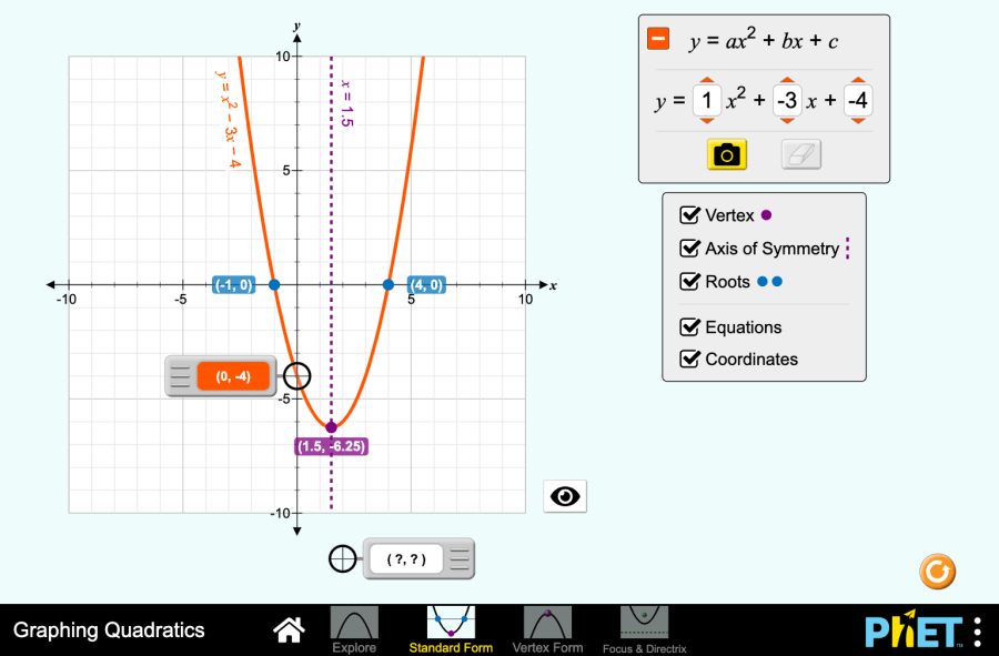
Objective: This virtual activity is designed for use in algebra lessons on the following topics: Theoretical part A function of type 𝑦 = ax2 + 𝑏𝑥 + 𝑐, 𝑎 ≠ 0 is called a quadratic function. Properties of the quadratic function: Parity: Increasing/decreasing: The graph of a quadratic function is a parabola. Elements of a parabola: Virtual experiment The Graphing Quadratics simulator allows students to explore the graph of a quadratic function. On the Explore screen, students can use the sliders to explore the effect of each term of the quadratic function on the graph of the parabola. The Standard Form screen focuses on the principal point, the axis of symmetry. Students can customize the function, but values are limited to integers.  Progression: Unit 1: Explore Step 1. Run the simulation: you will be presented with 4 different modes: Explore, Standard Form, Vertex Form, and Focus&Directrix. In this work, you will work with the first two modes. Run the Explore mode. Step 2. You are given: Step 3. a=1. Change this parameter differently. If you increase the value of a, the distance of the parabola will decrease, if you decrease it, you will see the distance increase. When you go to a negative value, the graph looks downward. Step 4. 𝑏=0. Change this parameter differently. If you increase the value of 𝑏, the parabola moves to the left the coordinate, if you decrease it moves to the right. Step 5. 𝑐=0. Change this parameter differently. If you increase the value of 𝑐, the parabola will move up the coordinate, if you decrease it, the parabola will move down. Step 6. Construct different equations and study their graph by changing the values of a, 𝑏, 𝑐. You can save and explore the graph types by clicking the camera button. Step 7. Try to explore the points of the parabola using the tools that show the point values (x,y) in the coordinates of the graph. Step 8. Open the equations section. Include the equations 𝑦 = ax2, 𝑦 = 𝑏𝑥, 𝑦 = 𝑐, and include the equations button. Examine the changes in the graph. Section 2: Standard Form Step 9. Go to Standard Form. You are given: Step 10. a=1. Change this parameter. Examine the changes in the graph.  In this section, the coefficients are represented as a natural number.  Step 11. Create different equations and explore their graphs by changing the values of 𝑏, 𝑐. Step 12. Try to explore the points of a parabola using tools that show the point values (x, y) in the coordinates of the graph. Step 13. Examine the coordinates of the graph by labeling the peak point, axis of symmetry, and roots. Step 14. Try adding equation buttons. The equation belonging to the graph appears next to the graphs.  Step 15. Do various investigations by changing the data in the equation. Conclusion The Graphing Quadratics simulator is a valuable tool for teaching students about graphing quadratic functions. The simulator has become interactive and visually useful by offering various tools for learning graphs such as displaying points, displaying equations, and saving graphs.

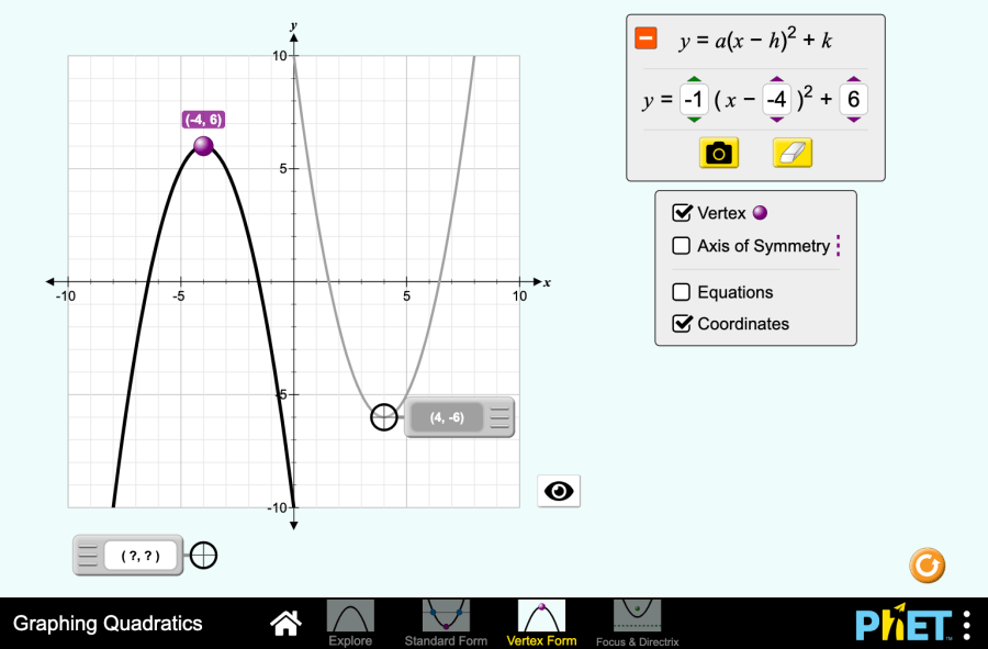
Objective: This virtual activity is designed for use in algebra lessons on the following topics: Theoretical part A function of type 𝑦 = ax2 + 𝑏𝑥 + 𝑐, 𝑎 ≠ 0 is called a quadratic function. The graph of the function y=f(x)+m is obtained by moving the graph of the functiony=f(x) vertically: The graph of the functiony=f(x+n) can be obtained by moving the graph of the function y=f(x) horizontally: The graph of the function y=f(x+n)+m can be obtained from the graph of the function y=f(x) by performing two consecutive moves: The standard form of a quadratic equation is as follows: ax2 + 𝑏𝑥 + 𝑐. The shape of the vertex of the quadratic equation is (a(x-h)2+k, where (a) is a constant that determines whether the parabola opens up or down, and ((h,k)) – are the coordinates of the vertex of the parabola. For example: The graph of a quadratic function is a parabola. Elements of a parabola: Virtual experiment The Graphing Quadratics simulator allows students to explore the graph of a quadratic function. On the Explore screen, students can use the sliders to explore the effect of each term of the quadratic function on the graph of the parabola. The Standard Form screen focuses on the principal point, the axis of symmetry. Students can customize the function, but values are limited to integers. On the Vertex Form screen, students explore the transformation of a parabola and identify the relationship between the graph of a parabola and a quadratic function. In the Focus&Directrix screen, students create a parabola based on the peak and focus. Progression: Unit 1: Explore Step 1. Run the simulation: you will be presented with 4 different modes: Explore, Standard Form, Vertex Form, and Focus&Directrix. Run the Explore mode. Step 2. You are given: Step 3. a=1. Change this parameter differently. If you increase the value of a, the distance of the parabola will decrease, if you decrease it, you will see the distance increase. When you go to a negative value, the graph looks downward. Step 4. 𝑏=0. Change this parameter differently. If you increase the value of 𝑏, the parabola moves to the left the coordinate, if you decrease it moves to the right. Step 5. 𝑐=0. Change this parameter differently. If you increase the value of 𝑐, the parabola will move up the coordinate, if you decrease it, the parabola will move down. Step 6. Construct different equations and study their graph by changing the values of a, 𝑏, 𝑐. You can save and explore the graph types by clicking the camera button. Step 7. Try to explore the points of the parabola using the tools that show the point values (x,y) in the coordinates of the graph. Step 8. Open the equations section. Include the equations 𝑦 = ax2, 𝑦 = 𝑏𝑥, 𝑦 = 𝑐, and include the equations button. Examine the changes in the graph. Section 2: Standard Form Step 9. Go to Standard Form. You are given: Step 10. Construct and study the graph of various equations by changing the values of a, 𝑏, 𝑐. In this section, the coefficients are represented as a natural number. Step 11. Try to study the points of the parabola using the tools that show the point values (x, y) in the coordinates of the graph. Step 12.Try adding the peak point, axis of symmetry, roots, and equations buttons. Examine the changes in the graph. Section 3: Vertex Shape Step 13. Go to Vertex Form. You are given: Step 14. Construct and examine the graphs of various equations by changing the values of a, h,k. In this section, the coefficients are represented as a natural number. Step 15. Try to explore the points of a parabola using tools that show the point values (x, y) in the coordinates of the graph. Step 16. Try adding the peak point, axis of symmetry, and equations buttons. Examine the changes in the graph. Section 4: Focus and Directrix Step 17. Go to Focus&Directrix. You are given: Step 18. Construct and examine the graphs of the various equations by changing the values of p, h,k. In this section, the coefficients are represented as a natural number. Step 19. Try to study the points of a parabola using tools that show the point values (x, y) in the coordinates of the graph. Step 20. Try adding the peak point, focus, directrix, parabola, and equations buttons. Examine the changes in the graph. Conclusion The Graphing Quadratics simulator is a valuable tool for teaching students about graphing quadratic functions. The simulator has become interactive and visually useful by offering various tools for learning graphs such as displaying points, displaying equations, and saving graphs.

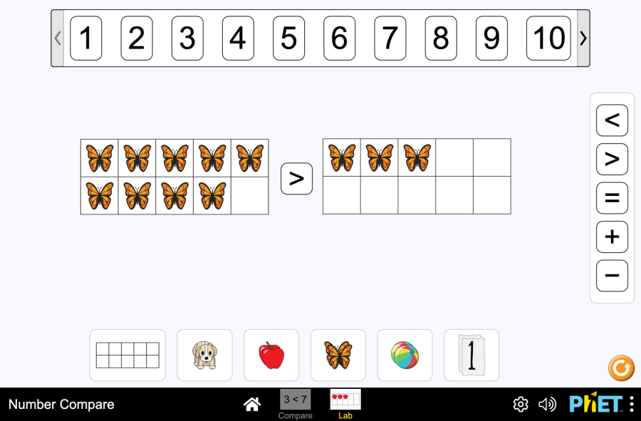
Objective: This virtual activity is designed for use in math lessons on the following topics: Theoretical part Comparing numbers is an activity that helps to determine which of two numbers is larger and which is smaller. Compare numbers by their place in the series of natural numbers. Compares two-digit numbers by digit, starting with the second (decimal) digit. If the number of decimals is the same, the units compare the digits. We compare numbers using comparison signs: Virtual experiment The “comparing numbers” simulation allows students to become familiar with and compare numbers. The numbers and pictures allow for flexibility in learning about comparison. Workflow: Part 1. Comparison Step 1. Start the simulation: you will be given 2 different modes, “Compare” and “Lab”. Open the “Compare” section. Step 2. Work area: Step 3. Place the puppy by holding down the left mouse button in window 1 for placing items. Step 4. In the windows above, you will see the result of the comparison: 1>0. Step 5. You can increase and decrease the number of items in the windows by using the buttons next to the object. Step 6. Place some puppies in the second window. Compare the comparison expression and the cube column. Step 7. Change the column of cubes to a segment type and observe the changes. Use a table so that the puppies are arranged in sequence. Step 8. Make several comparisons by placing the puppy in two windows to place items of different quantities. Step 9. Make comparisons by replacing the puppy with other types of objects (such as a butterfly or a number). Part 2. Lab part Step 10. Open the “Lab” section. In the work area, you are provided with: Step 11. Using the puppy and operations, create a comparison expression. Step 12. Compare the expression you created with the numbers at the top of the screen. Step 13. Additional Assignments: Conclusion Students learned how to compare numbers using virtual tools and modeling. The fact that the comparisons were not only in the form of numbers but also in the form of different objects made it easy for the students to understand the subject matter. This experience enriched the knowledge of mathematics and will come in handy in future learning experiences.